An Introduction to Probabilistic Programming

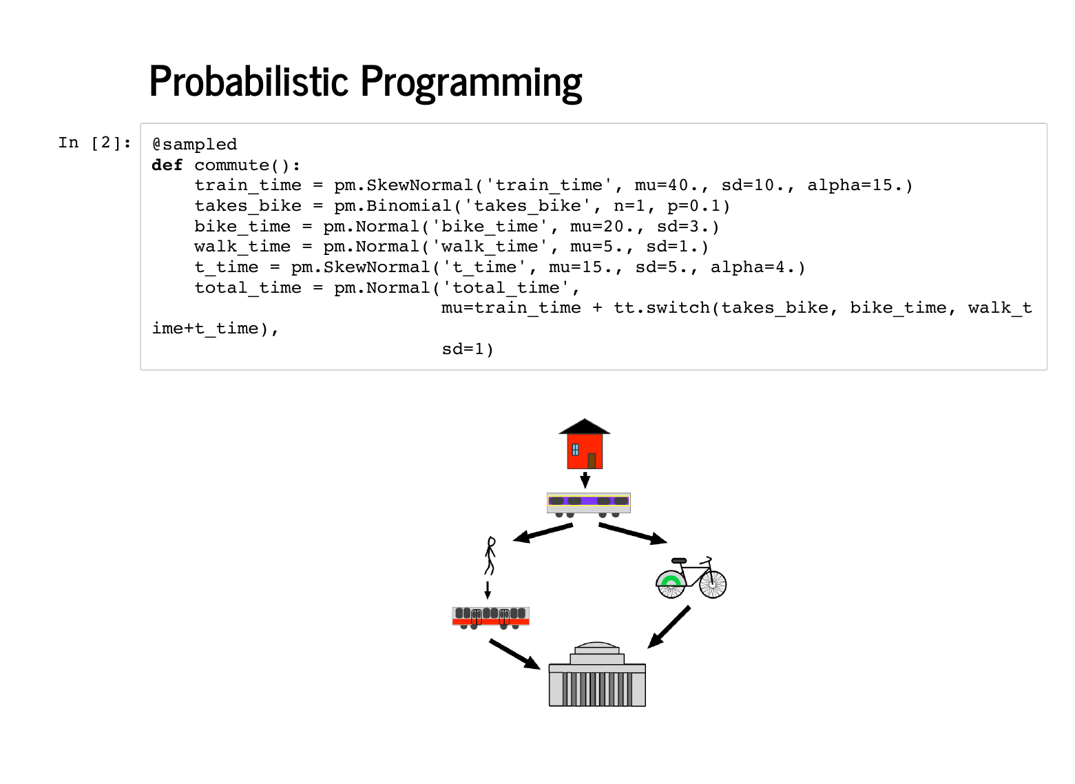
This segment concerns probabilistic programming, which has a technical definition and a whole literature around it. Given that we are at PyData, a mile or two from Columbia, and we got to see Dr. Sargent and Dr. Gelman's talks involving Stan, I want you to think of probabilistic programming as "what PyMC3 does." (Editor's note: Stan is great, and their devs have been extremely helpful in PyMC3 development.)

I have heard that New Yorkers love to talk about how to get from one place to another, so I am going to share my own commuting story. I wake up nearly in the mountains of New Hampshire and get on a commuter rail to Boston that usually takes 40 minutes. If it is nice, I'll take a bike after that, otherwise I need to walk from North Station to the Red Line, where I ride the T (subway) to Cambridge, where I work.

Here is that story implemented in a pymc3 program. We are also using a small library called sampled that so far has only been useful in talks. We will cover what it does later, but for now it just means that rather than using a context manager to define our model, we can use a function.

This is a beautiful, Pythonic approach to modelling. It is easy for a non-statistician to read, and we can look up the distributions we are not comfortable with to understand more about the model.

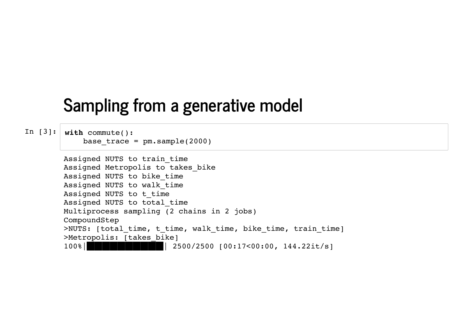
PyMC3's job though, is to sample from models. Everything in PyMC3 goes on inside a context manager, so you will usually see that wrapping the heavy lifting. In this slide, we are generating 2,000 plausible commutes, given the model we specified. This is called Monte Carlo simulation (note: not Markov Chain Monte Carlo), since we are still just sequentially randomly sampling.

PyMC3 is definitely not the best tool for this job - if such a simulation was our goal, we would be better off using Numpy's random number generators. It just so happens that PyMC3 makes it convenient to sample from the prior, so we might as well take a look.

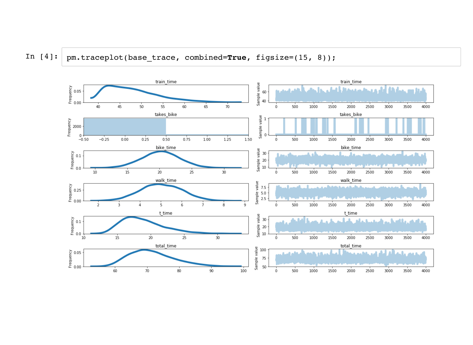
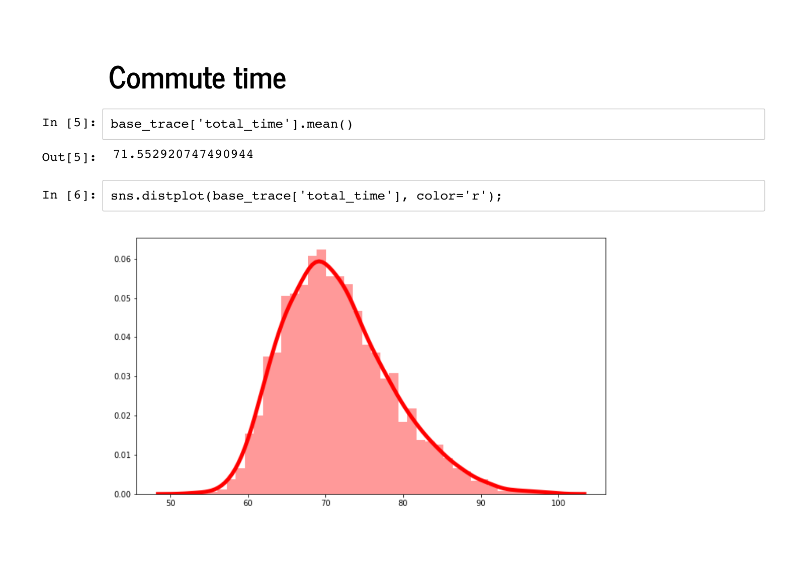
PyMC3 turns each variable in your model into an array of samples of that variable. This is a lot of data to handle, and the traceplot is a useful built-in visualization to get a handle on it all. On the left are individual histograms of variables so you can see, for example, that my average commute is just under 70 minutes. On the right are timeseries of individual draws, and you can see what point was sampled at each simulation. For example, takes_bike looks jumpy, because each draw is either a 0 or a 1.

We can also inspect the traces individually, since they are just numpy arrays. Note that they are of length 4,000 even though I asked for 2,000 samples. By default, PyMC3 will use multiprocessing to generate two "chains" of samples, since that is a best practice.

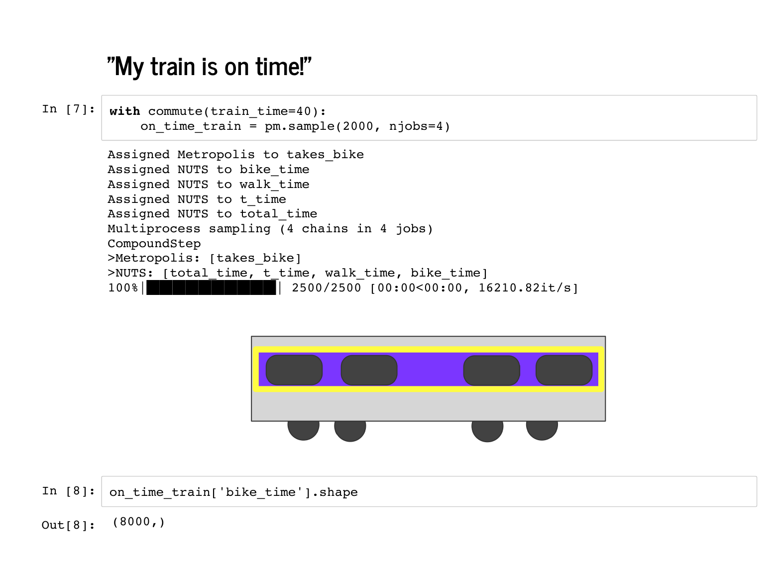
We mentioned that PyMC3 is not the best for Monte Carlo simulation, and you should use numpy for that. However, PyMC3 shines once we have more complicated distributions. For example, suppose I call ahead to work and say my train is on time. How does that change my expected arrival time? This is what sampled does well, by the way – it lets us reuse PyMC3 models, and pass in different patterns of observed data.

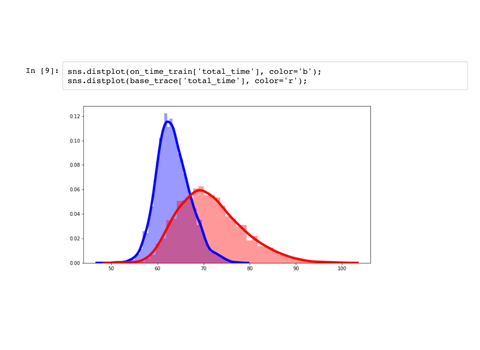
This is the distribution of my total commute time given that the train took 40 minutes to run. Notice that there is less uncertainty about when I will arrive, and usually I get there sooner than average.

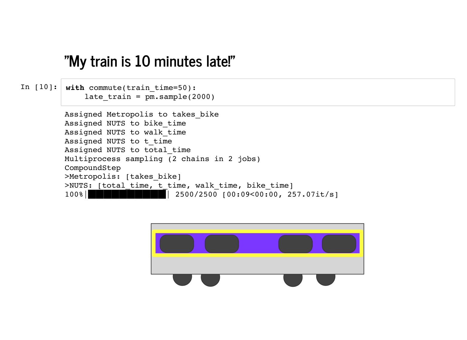
What if my train is late? In the same way as last time, I can sample from the distribution.

We again see a drop in uncertainty, but the whole curve is ten minutes to the right of the previous distribution.

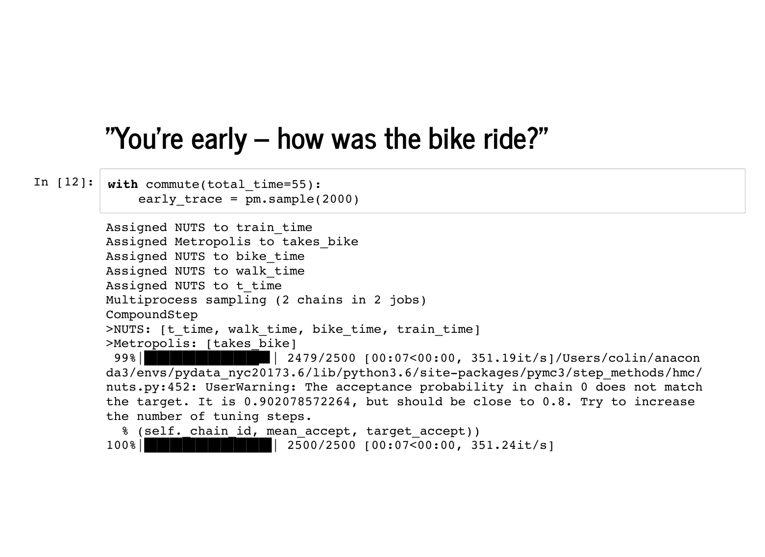
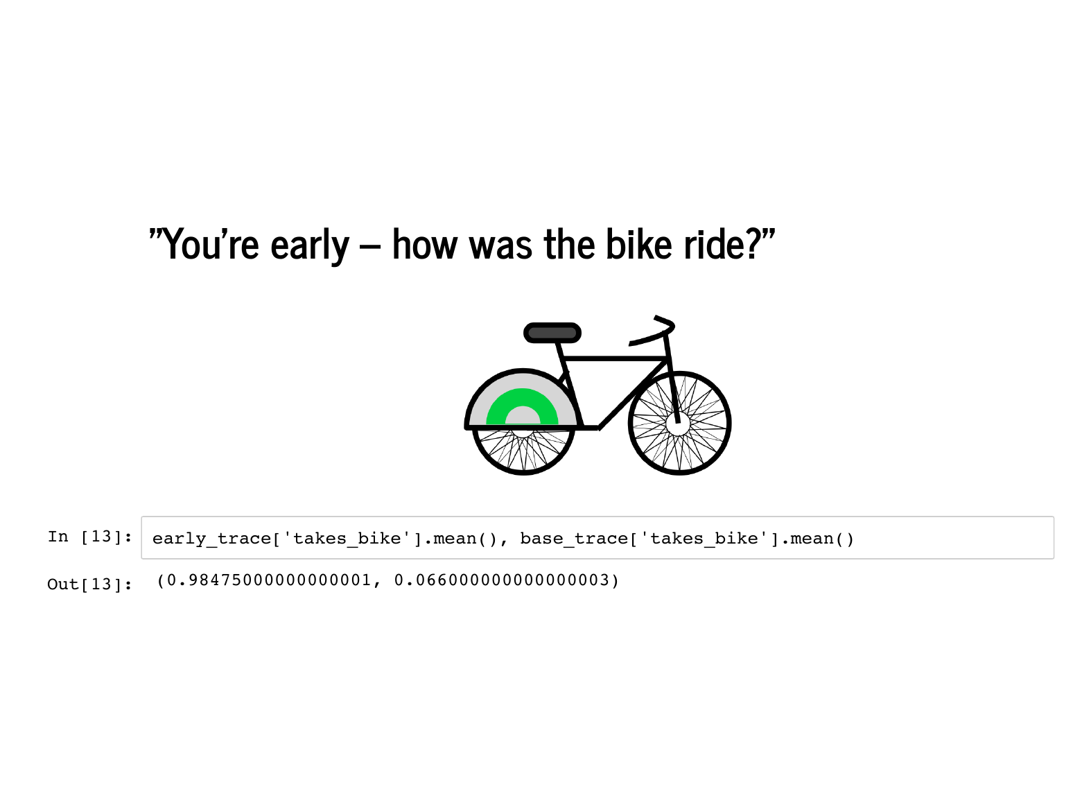
Now we will add observed data elsewhere. What if the total time it took me to get to work was 55 minutes? What might that say about my commute that day? Intuitively, we hope it says that everything was a little fast, or something was particularly fast.

One thing that comes out is that instead of our prior belief that I ride a bike 10% of days, we are almost certain I rode my bike.

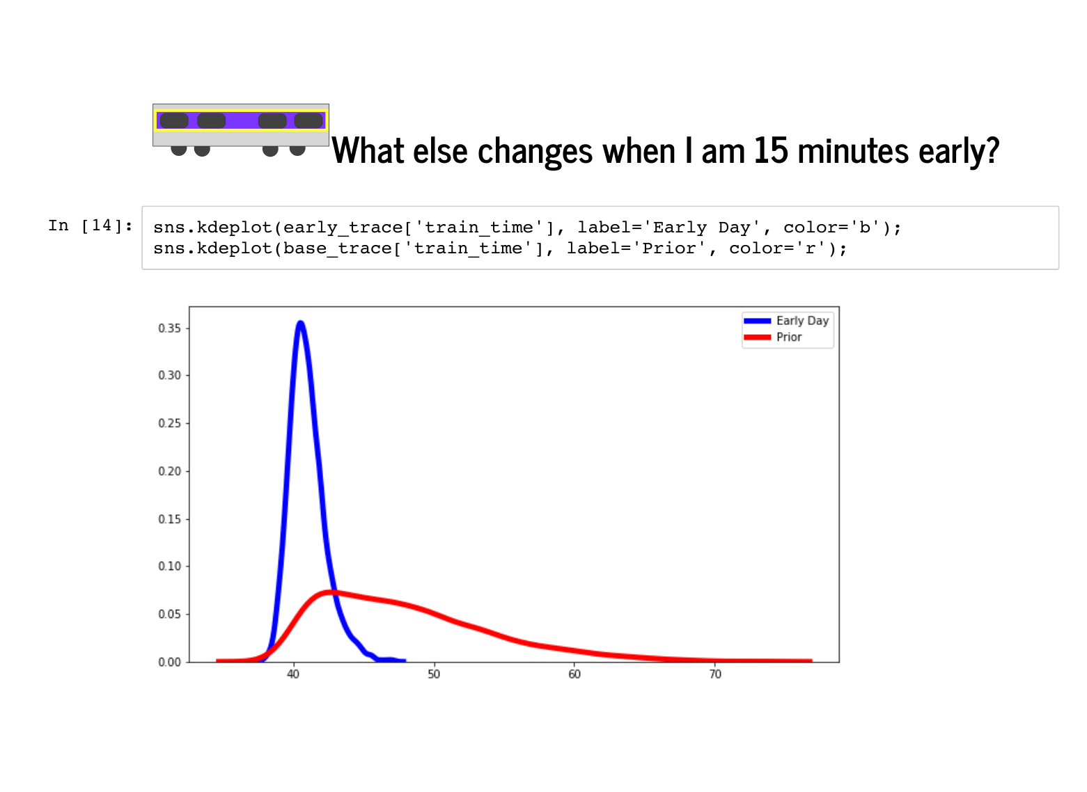
It also turns out that my train was almost certainly on time, and almost never more than 5 minutes late.

Once I got on that bike, I must have also really sprinted, going about 5 minutes faster than average.

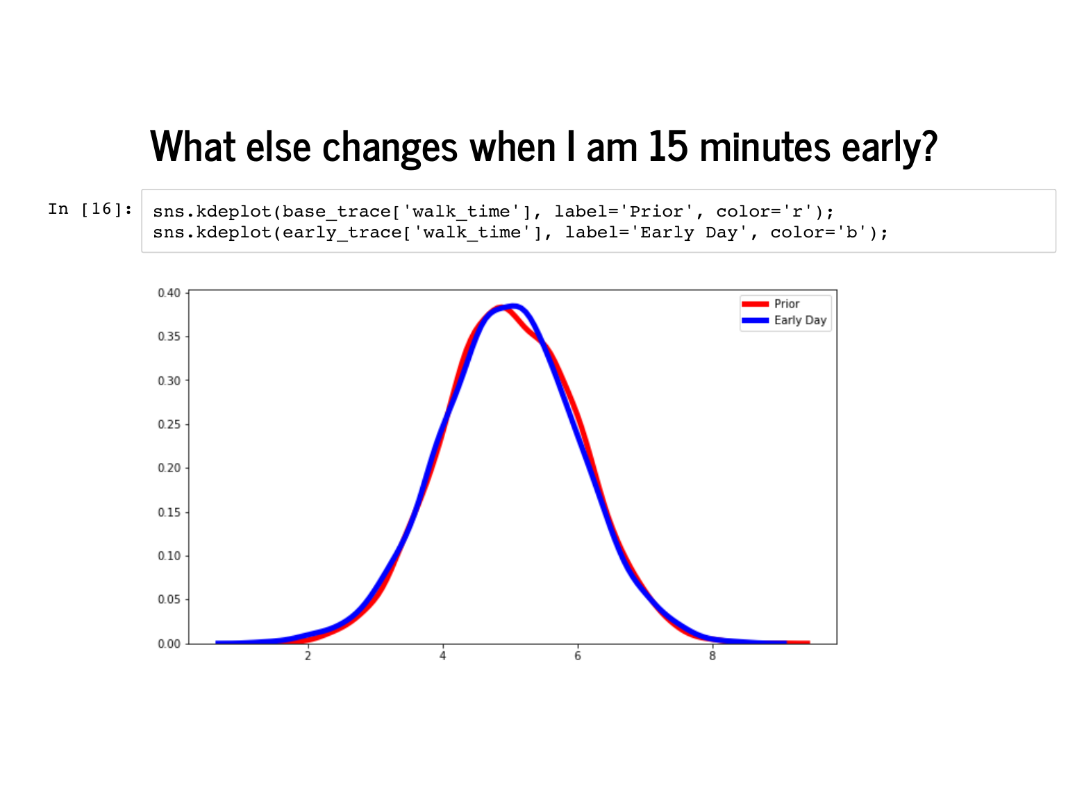
The shape of the walk time hardly changes at all, and that is mostly because I am usually taking a bike, so it does not matter how fast I would have walked that day. This is something to reflect on which is a bit of a problem with how we built the model. Whether I took a bike or the subway, PyMC3 sampled times for both modes of transit. The trace says that I took a bike almost every day, so we just ignore the subway time almost every day.

If we were being careful, we could have sliced the subway times by indices where takes_bike was 0.

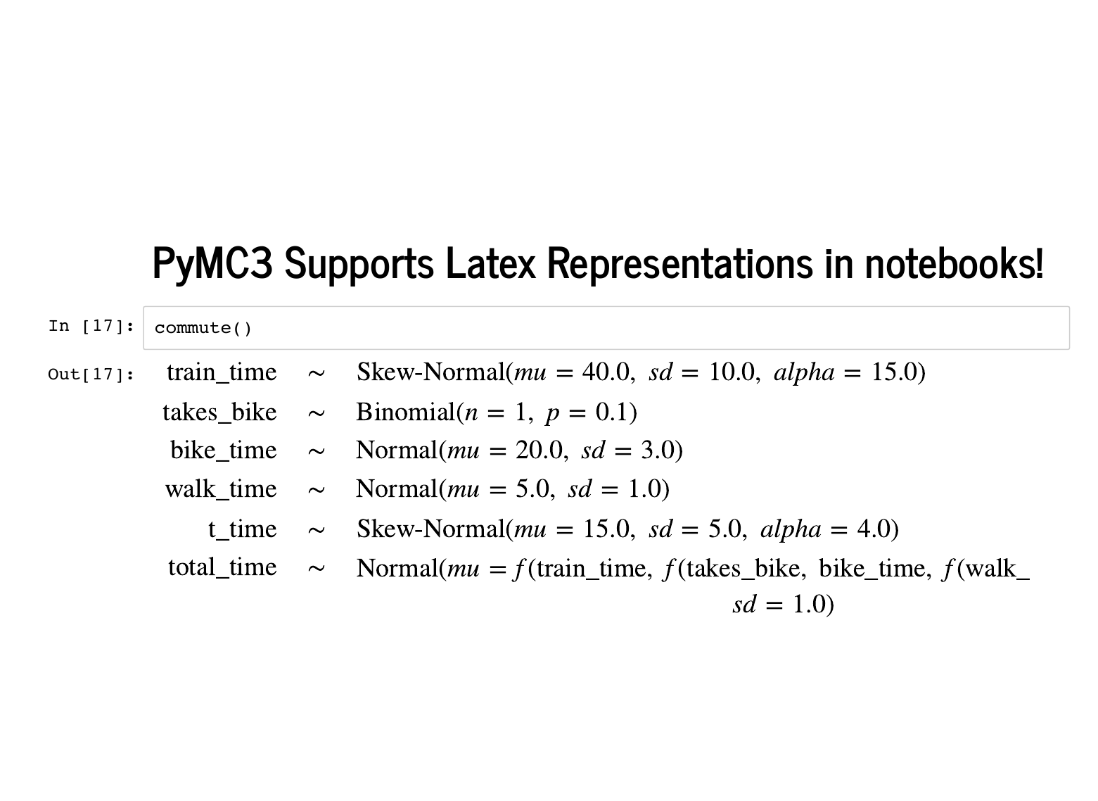
Lastly I want to quickly point out that in a Jupyter notebook, there is a nice representation of your model in LaTeX.