1. The Data
2. Linear Regression in Scikit Learn
3. Linear Regression in Numpy
4. Linear Regression with Regularization

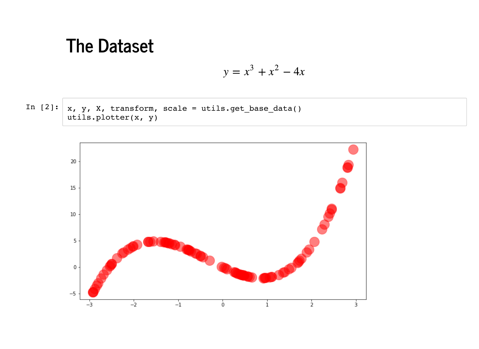
We are going to use a very non-linear dataset to practice linear regression. This polynomial provides a dataset that requires high dimensional features to fit, but can still be visualized in two dimensions. Specifically, there is a file in the repo called utils.py that will sample 100 random points between -3 and +3 to be our x data, and then pass it through f(x) = x³ + x² - 4x to generate our y data.

While generating the data and labels, we also generate the perfect feature vector, X, effectively telling our model that this is a 3rd degree polynomial.

There are a few downsides to fitting a polynomial, a major pain point being that they get very big very quickly, so the random seeds we are using are not random at all: I actually did a search to get a "good" random dataset. There will also be a few funny things we will do to take care of these explosions. A good example is the scale variable that we generate when generating data. This is a vector used to normalize the columns of features, and helps a lot with numeric stability, though we will not talk explicitly about normalization today. That scale vector will show up in a few places to do bookkeeping, along with the transform function.

Notice that this dataset is deterministic, meaning that we have not perturbed it with any noise. Any algorithm worth its salt should be able to recover this polynomial exactly, and our strategy today will be to fit algorithms first to this dataset, and confirm that we do ok here. In particular, we will make sure that each algorithm can recover the coefficients [0, -4, 1, 1].

After confirming we can recover these coefficients on the deterministic data set, we will want to see how our algorithm does on noisy data. We also “randomly” draw some normally distributed, standard deviation 1 noise that we will add on to this same dataset.

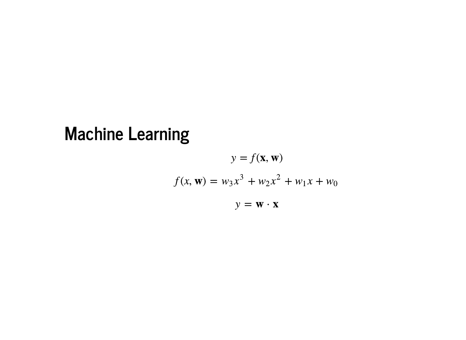
One way to think about machine learning is to write down a functional form for a model, and then design an algorithm so that the machine can learn the best parameters for that model. Following convention, lowercase italic "y" represents a single number, bold "x" represents a column vector and capital "X" represents a matrix, which is a vector of vectors. We also follow the convention that x are features, y are labels, and w are weights, or parameters.

It should be noted that your data are not your features. We are going to start with the simplest case, where we engineer our features to match how the labels were generated. Specifically, the labels are a third degree polynomial in x, so both w and x are vectors of length four. We can then use the language of linear algebra to write our model as just a dot product: y = x^Tw

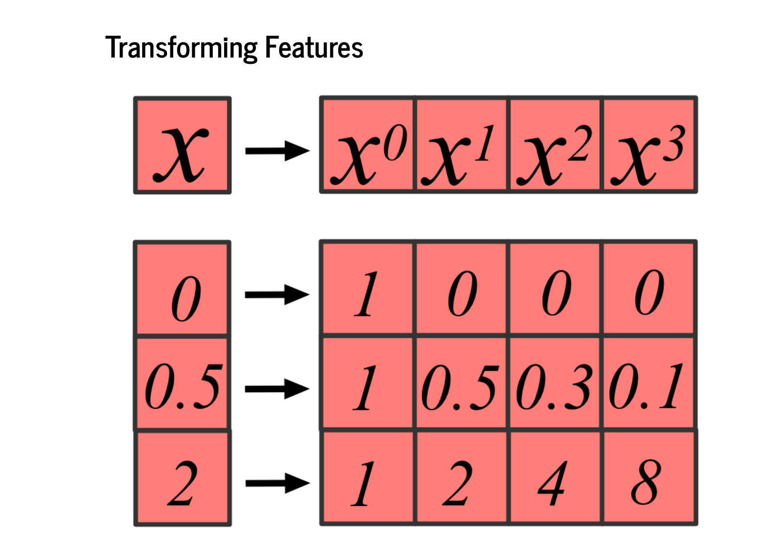
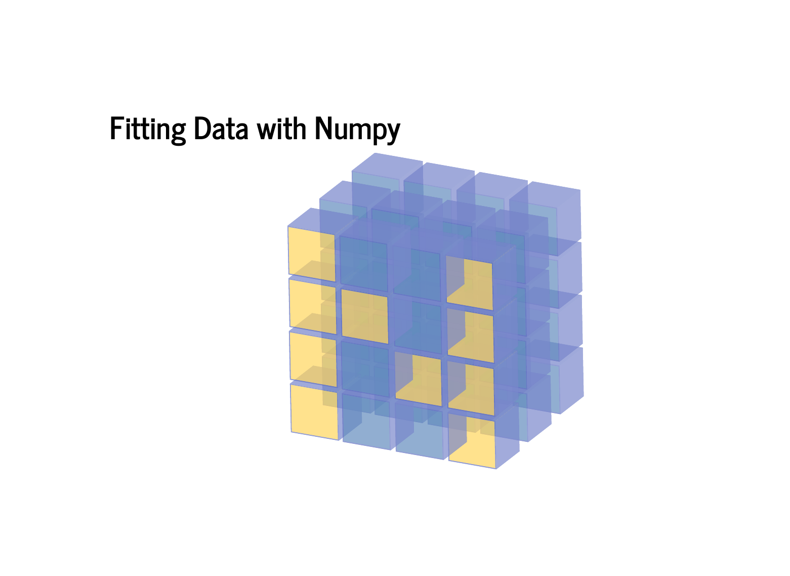
We will emphasize here that your data are not your features! Remember, our input data will be just a single number – a point on the x-axis – but we want our features to be that number to the 0th power, that number to the first power, second power, and third power. These are sometimes called basis functions, which transform your data into the features used to learn the model, and the basis functions can change the dimension you are working in. Here, we move from 1 to 4 dimensions.

The wonderful library scikit-learn will help guide us here, as it has so many others. The documentation for the library is a gem, and could serve as a course in machine learning on its own.

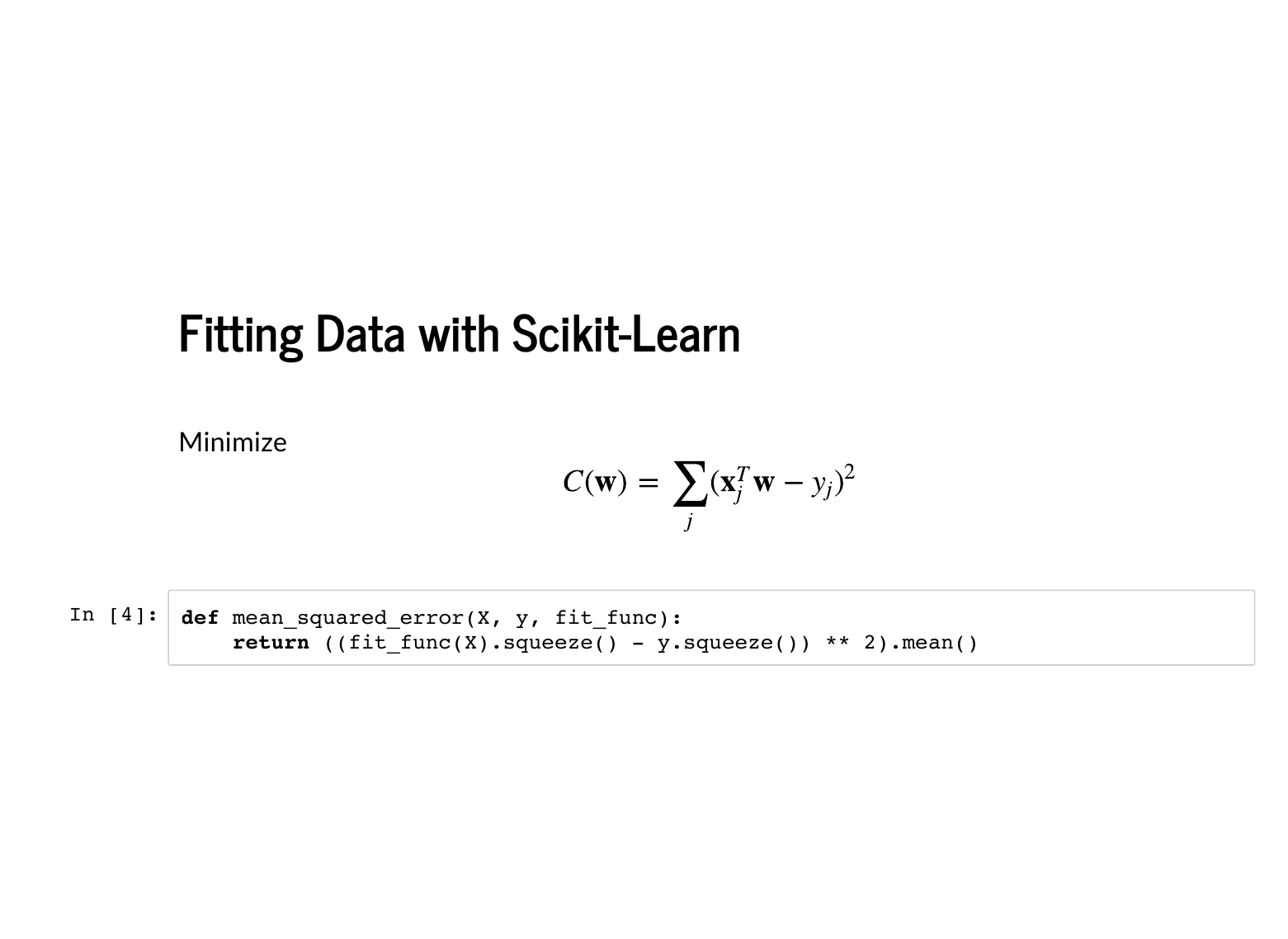
We are going to see today three ways of recovering the coefficients of our polynomial, each of which might be the high point of a different undergraduate math course, and each of which is made easy by a different NumFOCUS supported project. They are equivalent, so we can have a good argument over which math course, and which project go together, but I will argue that scikit-learn takes the approach from calculus.

Calculus is all about minimizing continuous functions. We said earlier that we want to find the "best" parameters, and scikit-learn does that by writing down the squared error, and minimizing it.

There's some matrix arithmetic we should look at here: x and w are both 4 x 1 column vectors, so transposing one and multiplying by the other gives us a 1 x 1 matrix, and we can subtract the number y_j from it.

Note that the squared error is not special to linear regression. Any regression model that makes a prediction can be scored with it. An emphasis of this workshop is that it corresponds to an assumption of normally distributed noise. We implement the squared loss in Python, and allow fit_func to be any regressor that outputs a number.

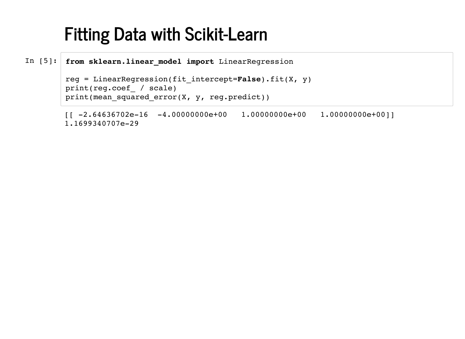
Python makes this easy: we can fit our model with one line of scikit learn. It is worth pausing to think how wonderful it is that there is a free project that allows that to happen with so little code.

Inspecting the coefficients, we can see we recovered [0, -4, 1, 1], as we hoped, and the mean squared error is 0, which is also great.

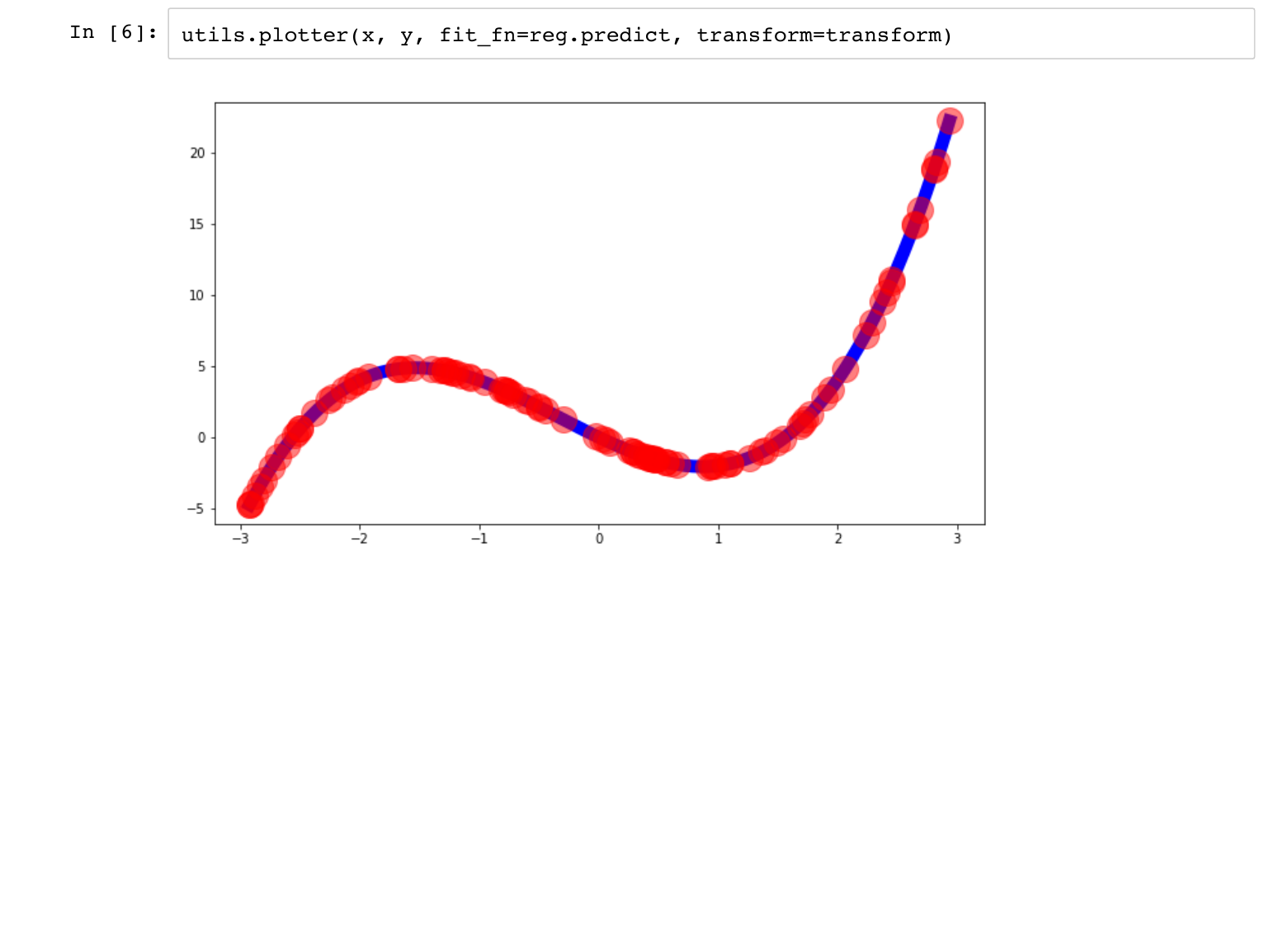
We can also inspect our fit visually, and see that we did great.

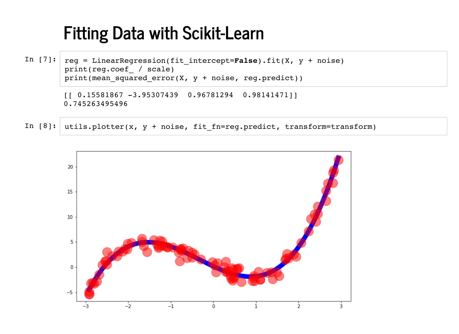
Adding noise to our data changes nothing about building our model. We are now wrong about the coefficients, but in some sense that we'll make rigorous later today, this is the best we can do. We specified our model exactly, but there's random noise, and this is the best model given the data: the true coefficients would have a higher mean squared error than this one.

We finished the calculus bit of the day, and it wasn't even that bad. We did not integrate anything, we did not take any derivates, and we have not seen any pictures of Pete. Now though, we get to the best part: the part where we do linear algebra with Numpy.

Linear algebra is my favorite subject in math. It is very appraochable, very tidy, and a good way to start learning proofs. If everyone watched Gil Strang's MIT Open Courseware lectures, the world would be a better place.

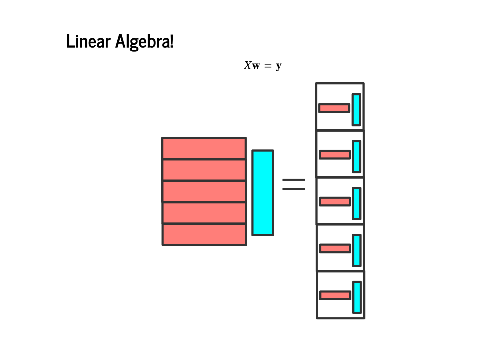
It is sometimes taught that you multiply matrices by multiplying row one by column one, then row two times column two, and so on. This approach is somewhat inscrutable, until you realize that the result is a vector of dot products. So when we have a feature matrix X, each of whose rows is a feature vector, our linear model is the matrix product Xw = y.

Earlier, we wrote our model as 100 dot products of features and weights, and now we are just "vectorizing" that over the entire set of features and labels.

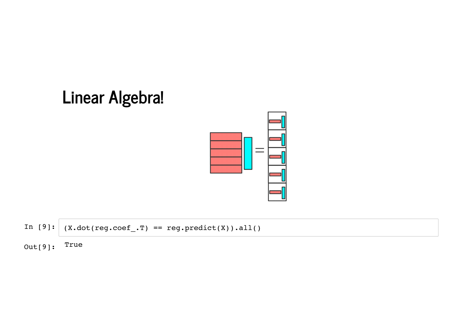
We can even confirm that this works using the scikit learn model we fit earlier. Multiplying the features by the learned coefficients gives us exactly the same predictions as calling the .predict method. This is not a proof, but it is at least nodding suggestively that it might be true.

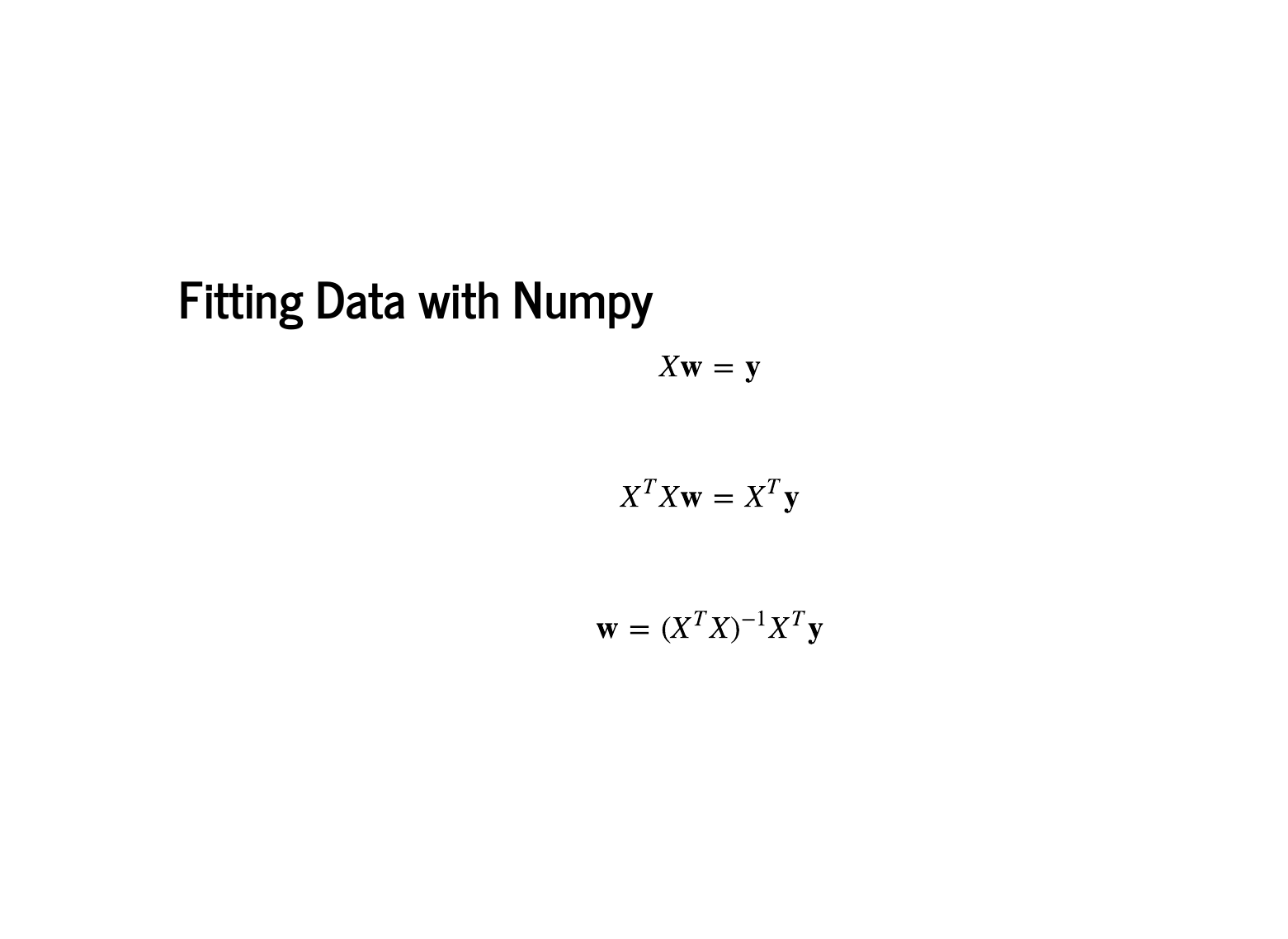
So how can we fit a model with just numpy? We have built up the problem a little bit, but we ought to just try to solve this. We have an equation here, so it is natural to just multiply by X^-1 on both sides.

The problem with that approach is that X is a rectangle – it is likely tall and thin – and only square matrices can even have inverses.

Also, scarfs are for people, not dogs, but Pete looks great.

So we try again. This is a common "trick" in linear algebra that has beautiful geometric intuition you can ask Gil Strang about: we multiply by the transpose on both sides. If our matrix X was 100 x 4, then X^TX will just be 4 x 4. It will also probably have an inverse, and we will not worry about the case where it does not.

This big matrix (X^TX)^-1X^T is called the Moore-Penrose pseudoinverse. The derivation on the slide is the only way humans know how to remember the equation, and I would encourage you to memorize it too.

It has a subtle lie in it, though: it is not true! Typically we will not fit a line exactly, so there's no w so that Xw = y. Then it should be concerning that we found a w that claims to solve the equation. Inspecting closely, the very first equals sign is full of lies.

Thankfully, the w we derive and the Moore-Penrose pseudoinverse still satisfy some nice properties. An easy one is that if the equals sign is not a lie, then we will recover the correct w.

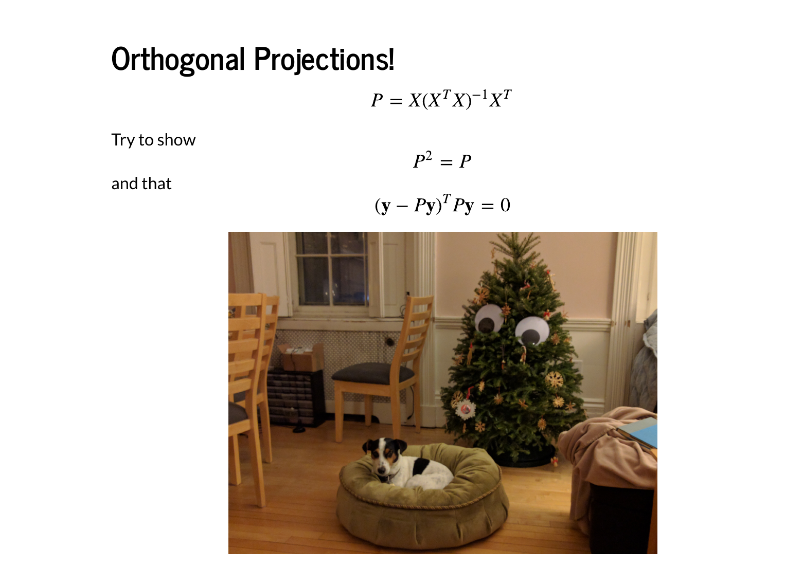
Optional math heavy slide

In particular, P = X(X^TX)^-1X^T is "an orthogonal projection matrix onto the column space of X". This means that Py is the closest we can get in a high dimensional space to y, given the data. And this is "closest" in the Euclidean distance sense, which is exactly the sum of squared errors!

The slide has two super-bonus questions for the linear algebra junkies. We confirm two properties of this matrix: Itempotence is a concept that is beloved in software engineering, ane means that applying the function twice has the same effect as applying it once. Orthogonality means that the dot product of y with Py is 0.

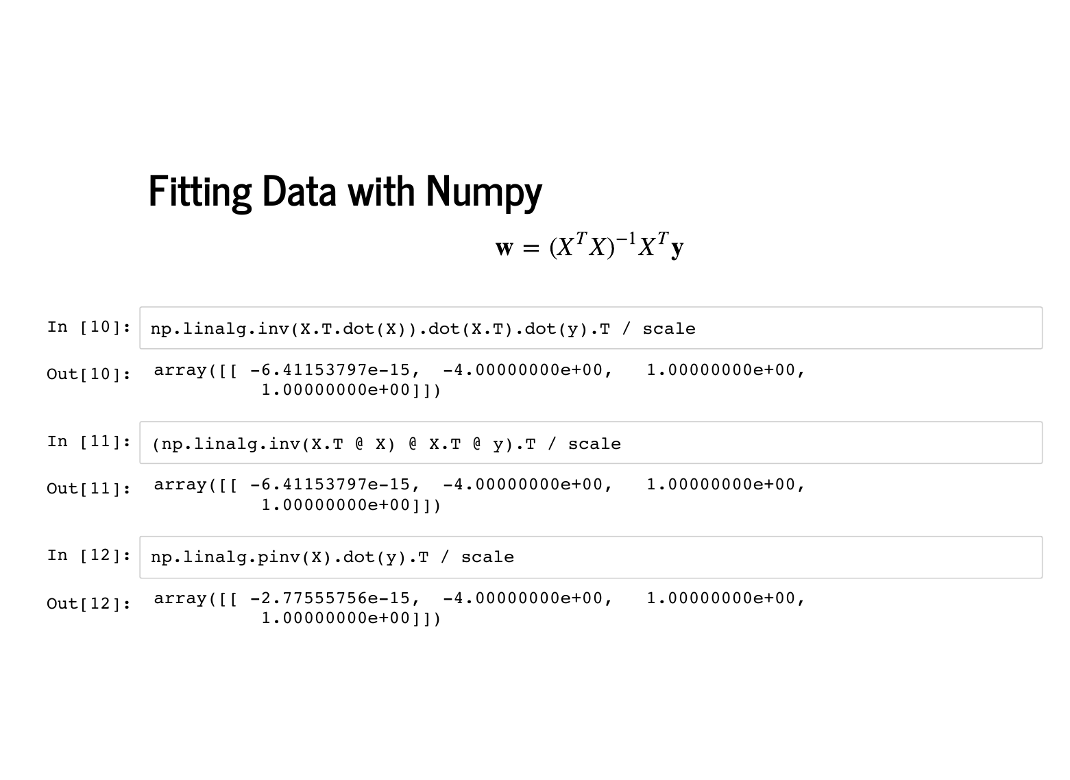
Back to writing code, though! Numpy is wonderful because we can just write down the Moore-Penrose pseudoinverse, and recover w, using chained methods.

When using modern Python, in particular since 3.5, you can also write it with the @ operator, which is a certain kind of nice.

Finally, this is such a useful matrix that numpy even has it built in, with some extra numerical stability, so we will use this one. Note that "pinv" stands for "pseudoinverse", so it is anyone's guess how to pronounce it.

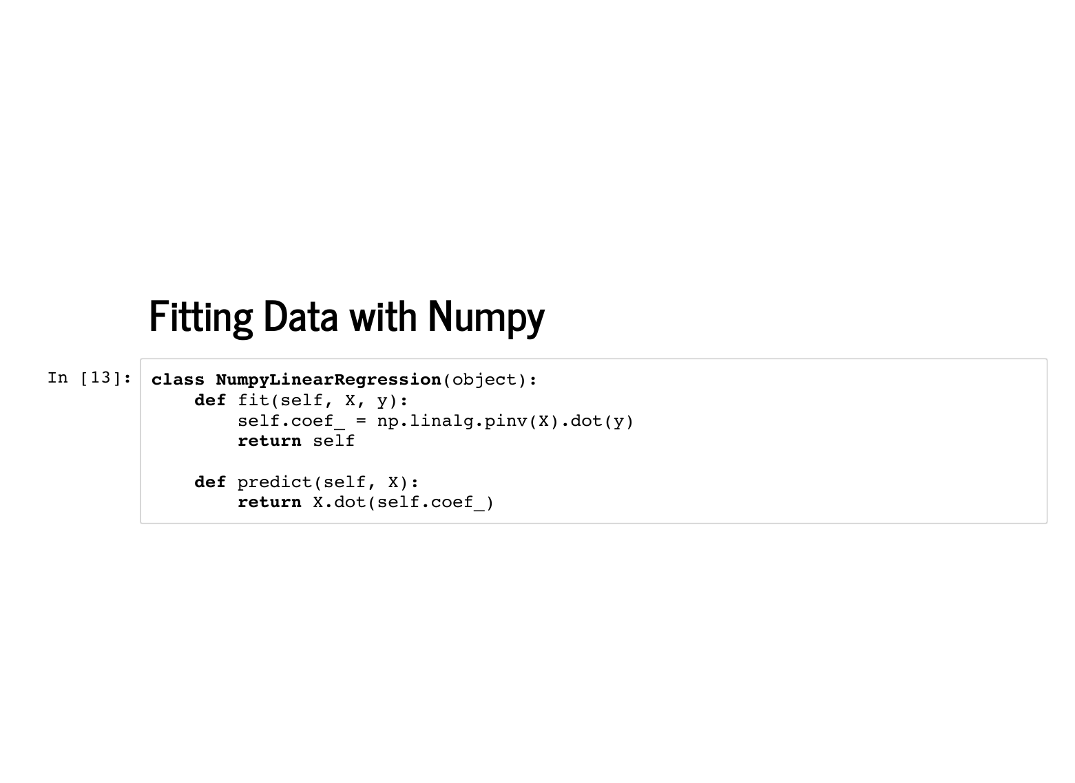
We are also going to keep emulating an sklearn API. This will let us reuse a lot of code, and make what we write a bit easier to grok. This slide has our minimal implementation of linear regression. Note we just use pinv to fit our coefficients, and then use matrix multiplication to make predictions.

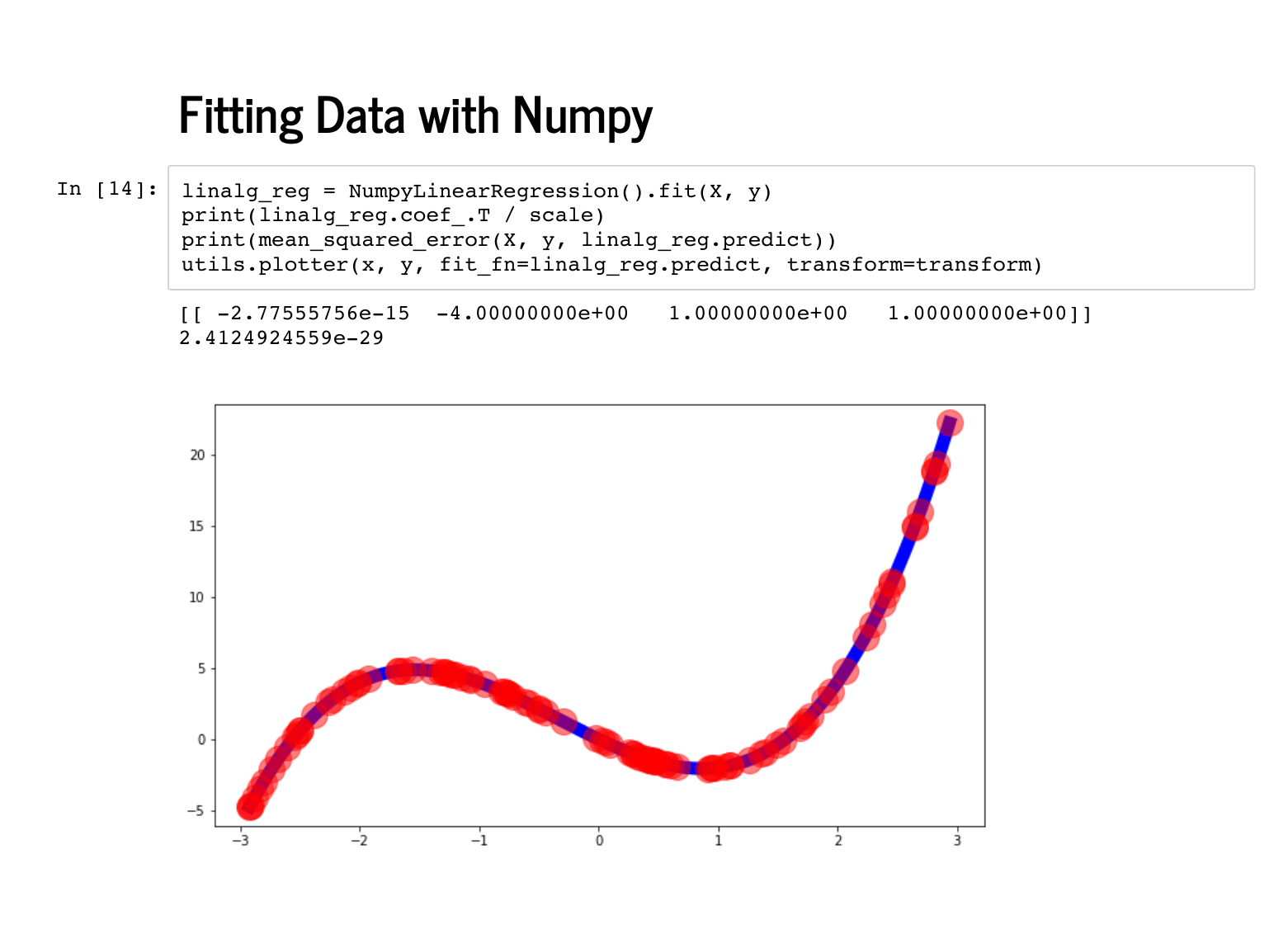
Now we can use this with the exact same lines of code as our scikit-learn regressors, and it has the exact same fit that those had.

The noisy version, too, is straightforward, and gets the same coefficients back.

The last thing I want to talk about is regularization. I am going to use a proper train and test set here, though a little imbalanced: 20 points to train, 80 points to test. Note that with the proper features, fitting this polynomial is still not very hard. But now instead of 4 features for a third degree polynomial, my features will have 15 dimensions and end up fitting the data too well.

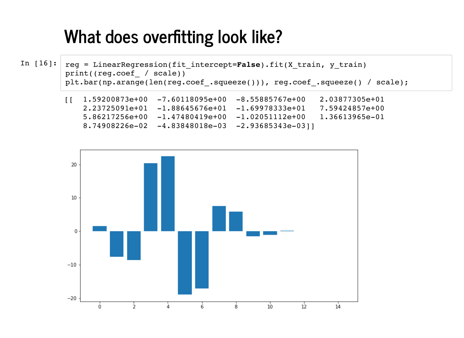
It is a little harder to glance at all the coefficients, but this bar chart shows that the first four coefficients are not particularly close to the [0, -4, 1, 1] that we expect, and the last 11 are not uniformly close to 0.

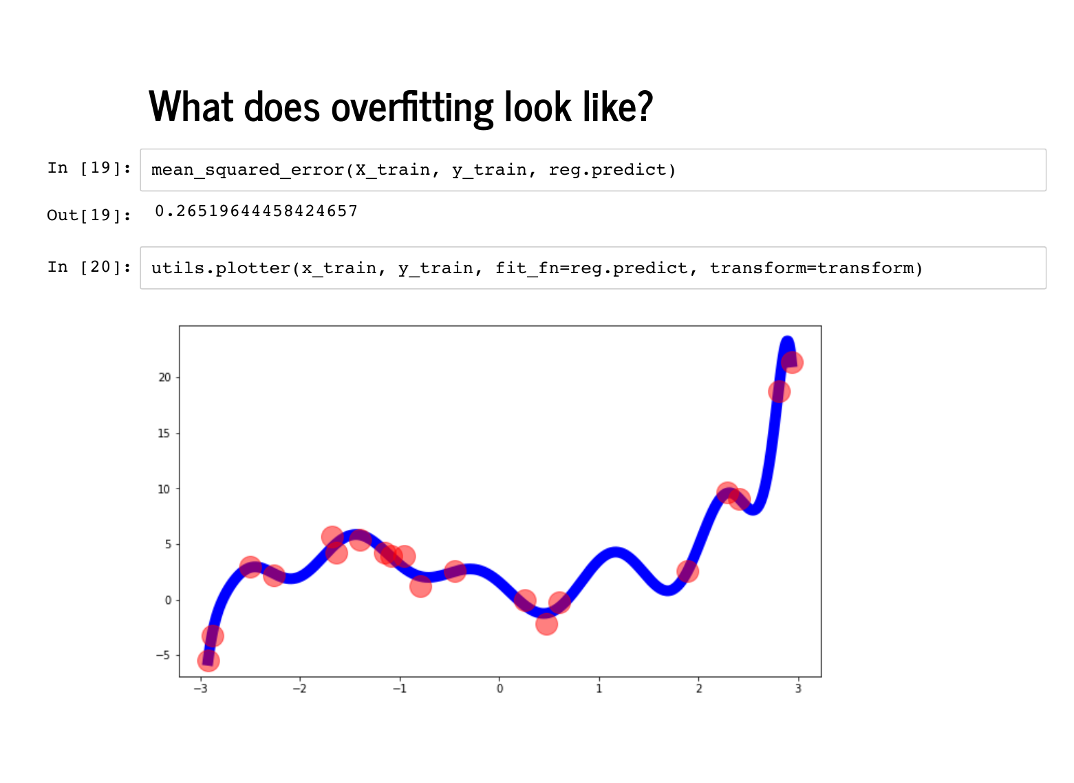
The plot also looks quite wiggly (technical term), and even though the mean squared error on the training set is quite low, the error on the test set is quite high.

This is called overfitting, and can happen when there are too many irrelevant features. Adding an extra feature will always improve your performance on the training set, but may degrade performance on a test set. This is a common problem with feature engineering: it can be hard to know ahead of time what the relevant features will be!

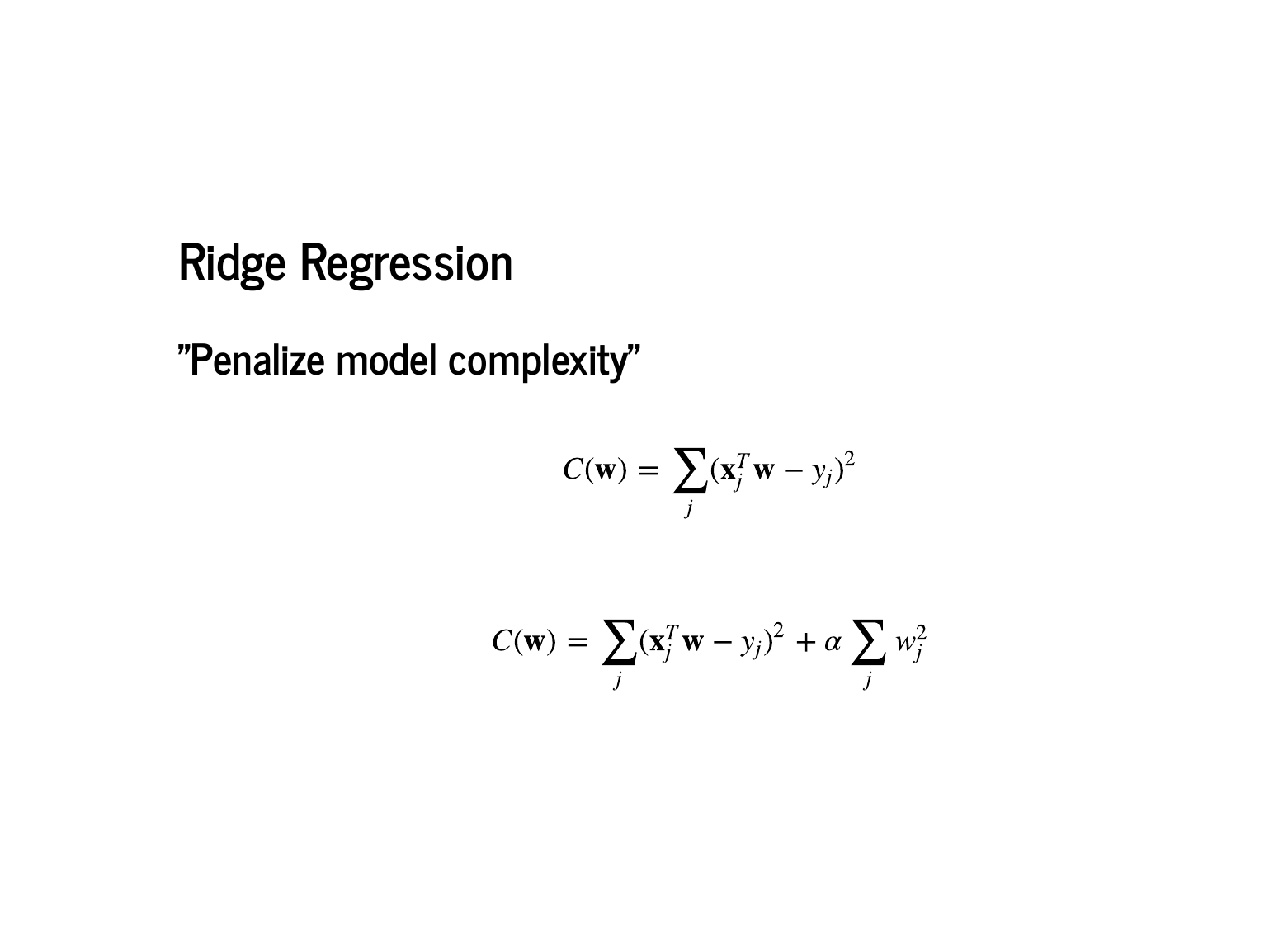
One way we try to deal with overfitting is by penalizing model complexity.

In particular, we add a penalization term to the cost function, and find weights that minimize this new function instead. Note that alpha is now a parameter we may need to fit, and it controls the strength of regularization. Using the sum of the squared weights is called Ridge regression, or l² regularization.

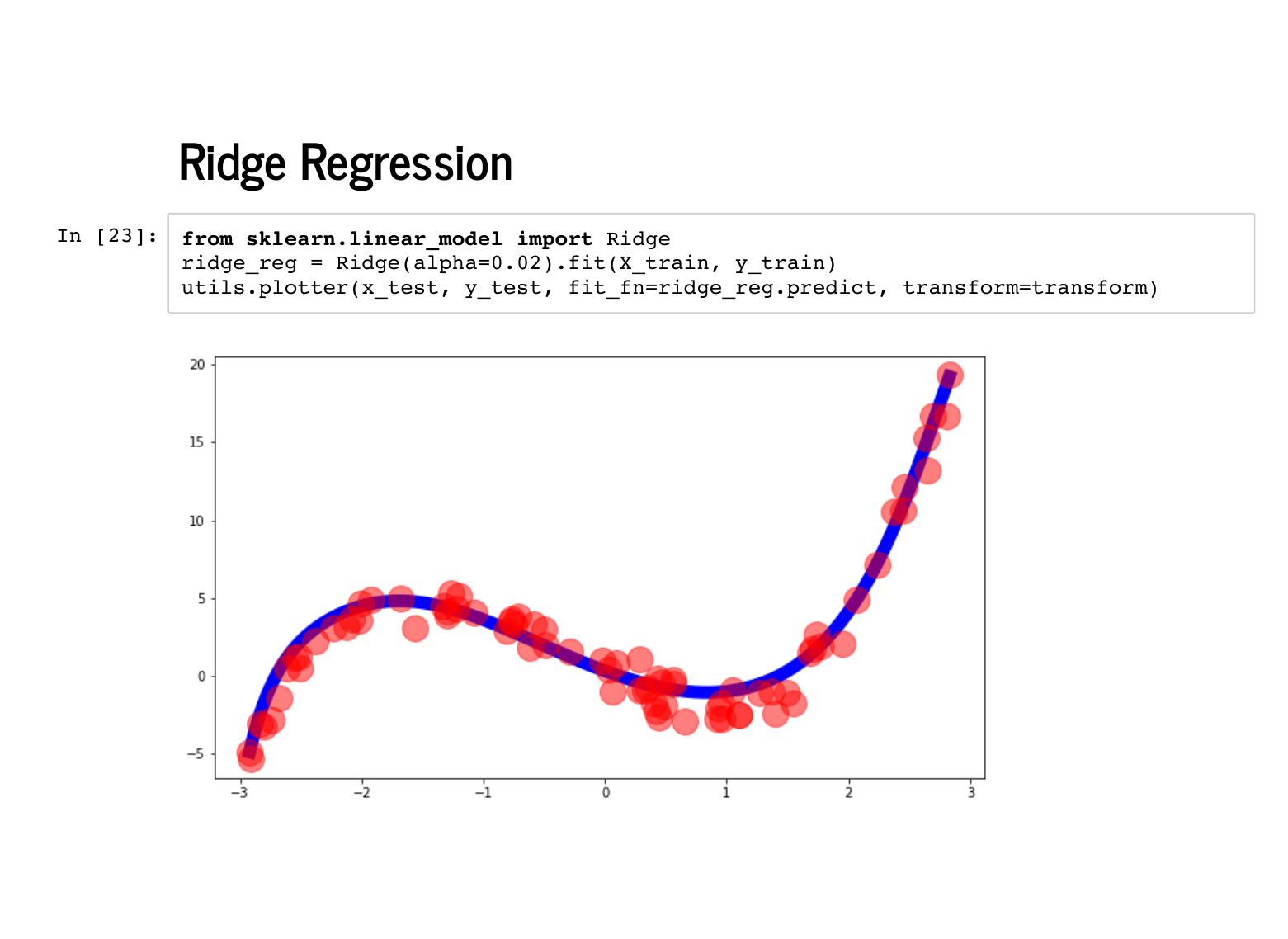
Sklearn makes ridge regression just as easy as normal linear regression.

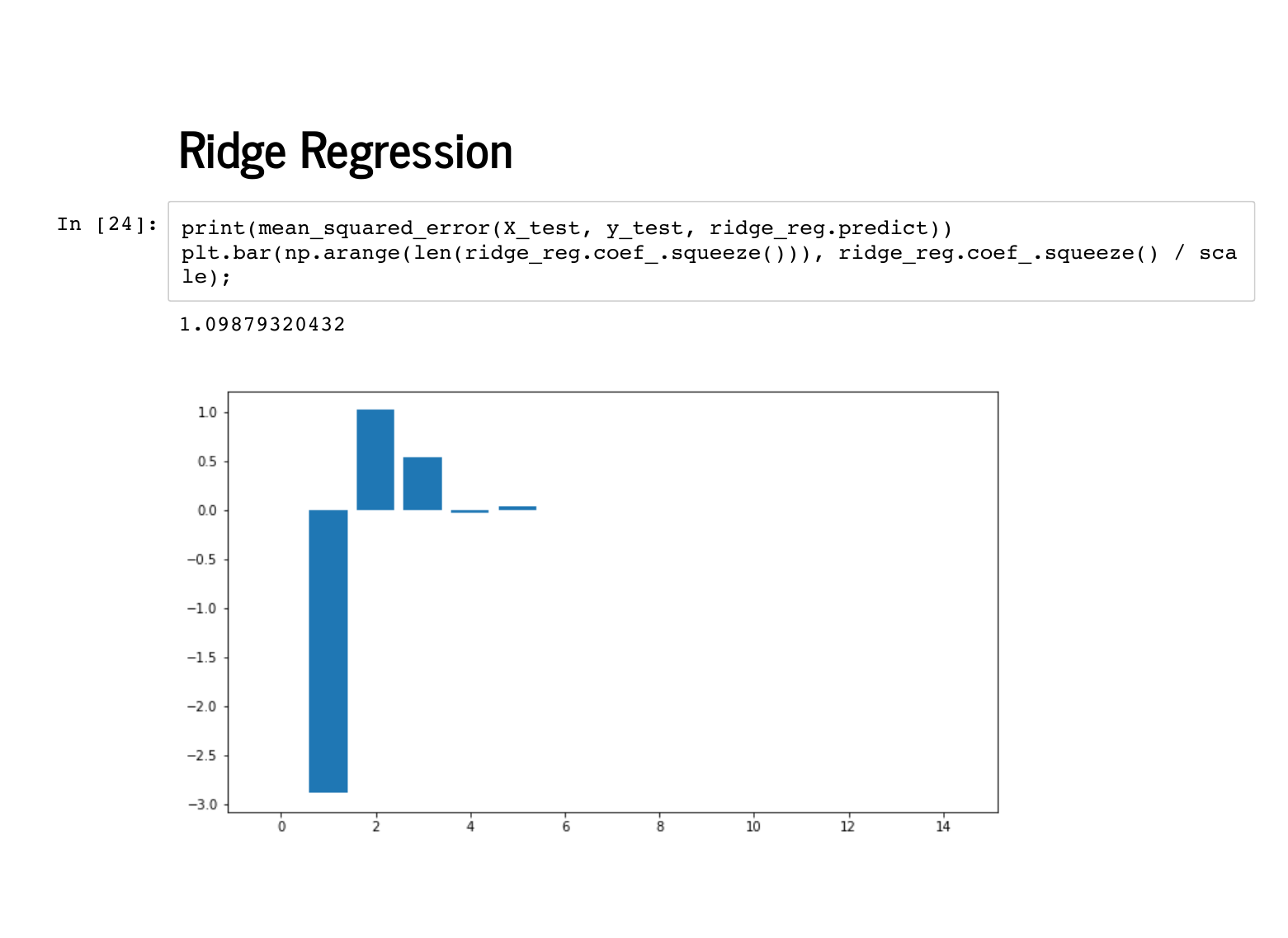
The coefficients it learns are even plausibly near [0, -4, 1, 1], followed by eleven 0's.

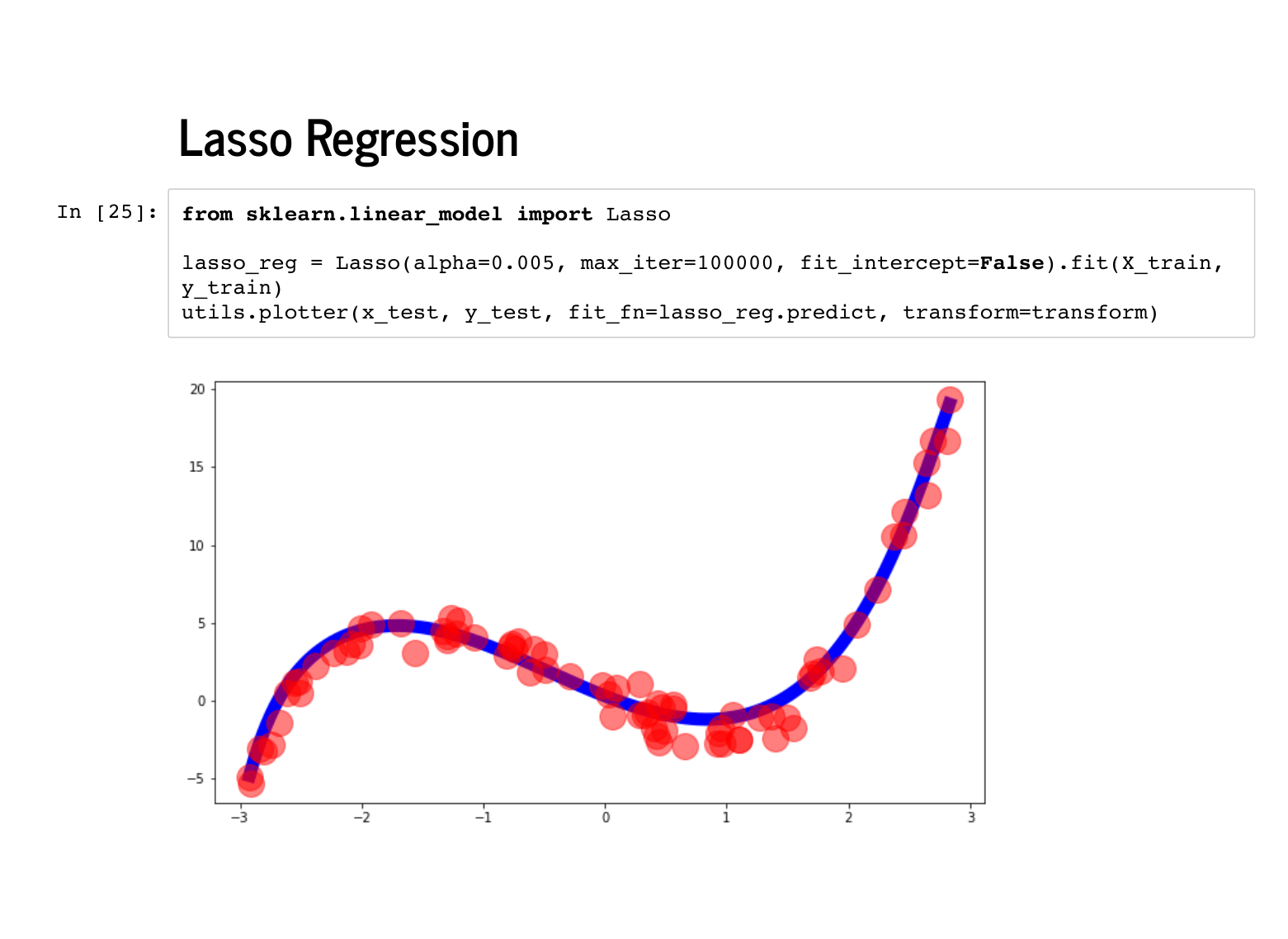
Lasso regression, or l¹ regularization, means we penalize with the sum of the absolute value of the weights. It is also quite easy with scikit learn. For technical reasons, it may require some extra arguments, like max_iter here.

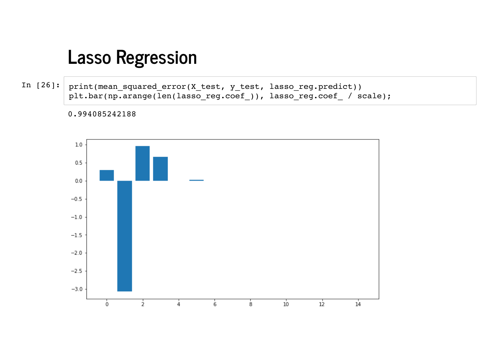
Lasso is beloved for encouraging sparsity – coefficients that are exactly 0 – instead of just encouraging them to be small, like in ridge regression. You an see that these weights are also quite near [0, -4, 1, 1].