1. Bayesian Linear Regression
2. Bayesian Ridge Regression
3. Bayesian Lasso Regression
4. Conclusion

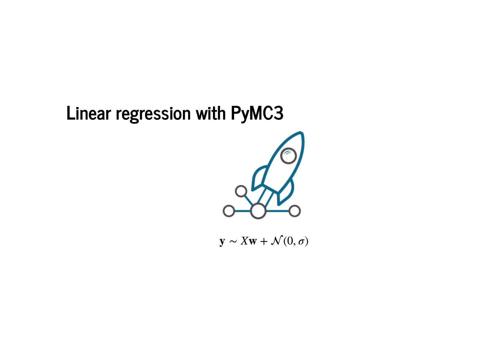
For the last bit of the workshop, we will talk about linear regression with PyMC3. There will be linear algebra, there will be calculus, there will be statistics. Physics is awkwardly in the background, saying hi to Pete the pup.

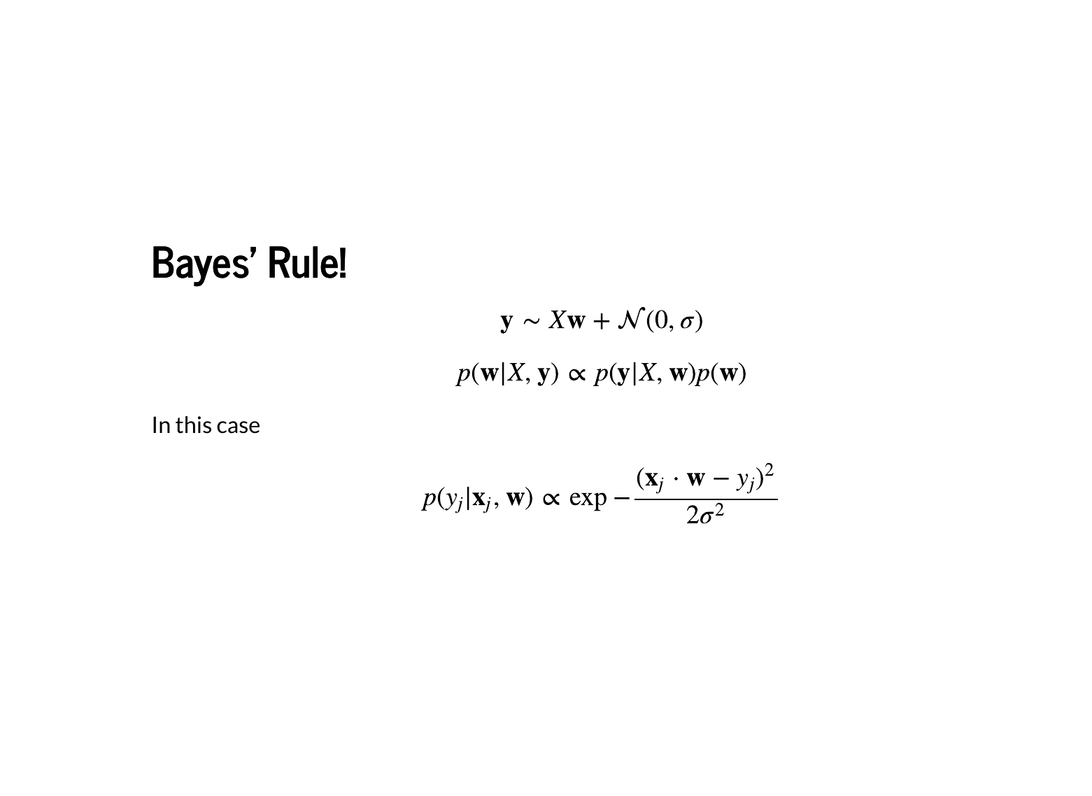
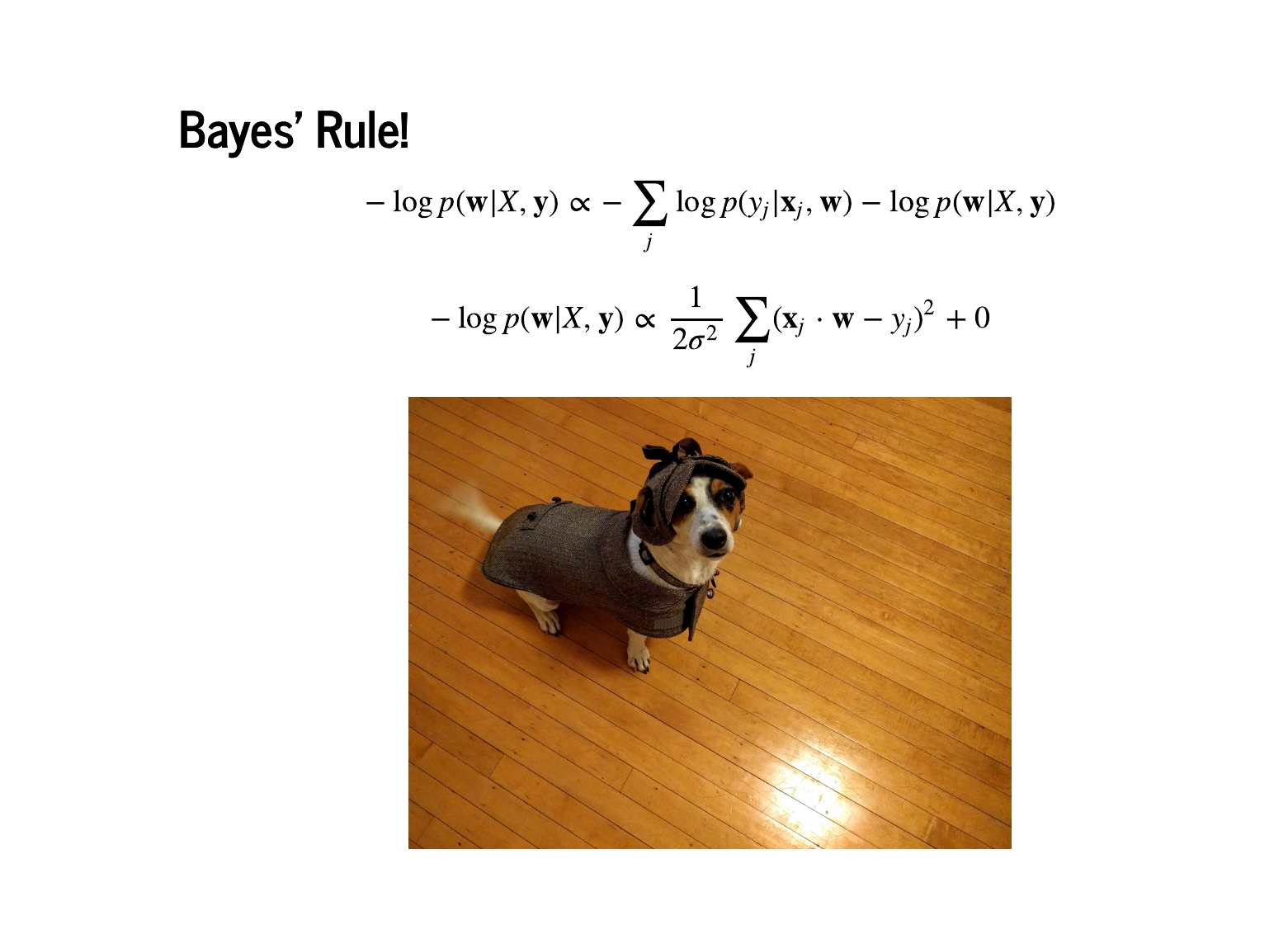
Our goal now is to model how the data is generated. But we know how the data was generated: we added some normally distributed noise to the data.

We know that we are doing some serious work now, because these equations are joined by two different operators that are not "=", ">", or "<". The "∼" means that the items on the left and the right are probability distributions, rather than a single value. If we were being careful, distributions only make sense under an integral sign, but this is useful shorthand.

The "∝" means "proportional to". This means there is some quantity that I am claiming will not matter to the calculuation, but I encourage you to not trust me and do the bookkeeping of constants yourself.

In this case, we are modelling the labels y as being normally distributed around Xw, for some w. The last equation on the slide is the normal distribution's probability density function. Plugging in values for x_j, y_j, and w will let us evaluate the probability of any single point.

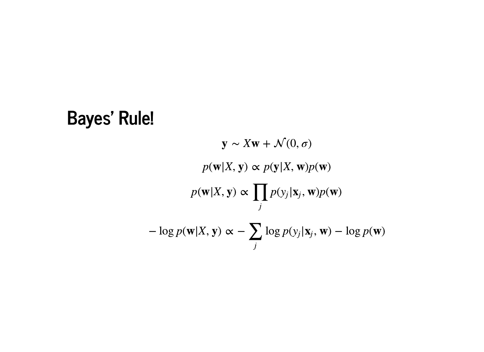
Now these are some equations! Before diving in, we should step back and just admire this. Greek letters, underscores, no Python code at all. We will get to some working code soon, so Dr. Sargent does not think we are bullshitters, but for now we should just revel in this for a moment.

Bringing this back into focus, the first two lines are from the previous page. They are our modelling assumption, and Bayes' rule. The third line is our assumption that the data is independent, so the probability of all the data is the product of the individual probabilities.

Finally, we take the negative log of the whole thing. This is nice from a numerical point of view: the product of a bunch of numbers less than 1 is going to be very small. So we turn that unstable product into a sum of numbers that are greater than 1. Also, the log is a monotone transformation: if we maximize the log of a function, we have also maximized the function. The negative sign lets us find a minimum instead of a maximum, which is a pleasant convention.

Now all this holds for any probability distribution. Note that this sum comes from our likelihood, and the term on the right is called our prior. What happens when we plug in the normal distribution for our likelihood?

The exponential and logarithm cancel each other out, and we are left with minimizing the sum of squares. That means the maximum a posteriori estimate will be exactly the set of weights that sklearn gives us! This is, of course, assuming that statistics, linear algebra, python, sklearn, and PyMC3 all work correctly.

Also look at Pete. He thinks he is a detective!

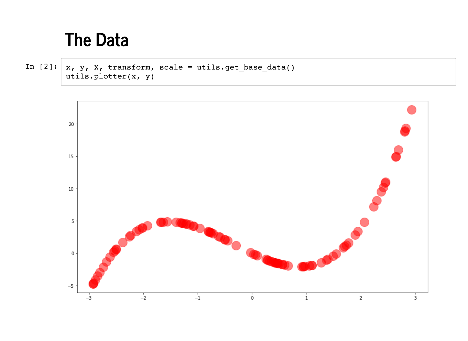
We should use this model, and confirm that all these fields and software libraries are indeed correct. Here is the exact same data set that we used at the start of the workshop.

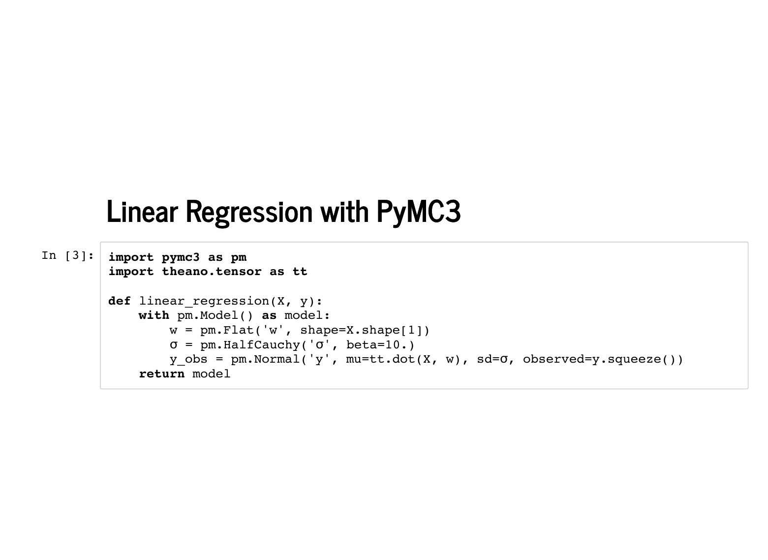
This is our linear model. We put an improper prior on the weights, so that any set of weights is equally likely. We fudge a little and put a prior on the standard deviation to avoid some problems in sampling a model with no noise. Finally, we define our likelihood in the last line. The function returns a PyMC3 model, which can be used as a context manager, so we can write some slick code.

Here we go! The sampling step actually is a little tricky because there is no noise: if a positive standard deviation is sampled, it ends up having very low probability.

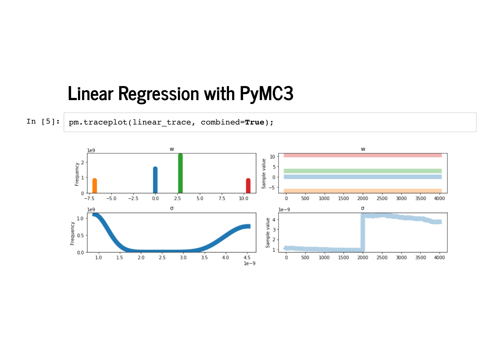
The trace plot looks a little funny, but notice the scale on the standard deviation is 1e-9, and our probability distributions for the weights are really just point masses. This is a funny thing to model with continuous distributions, but PyMC3 does okay with it.

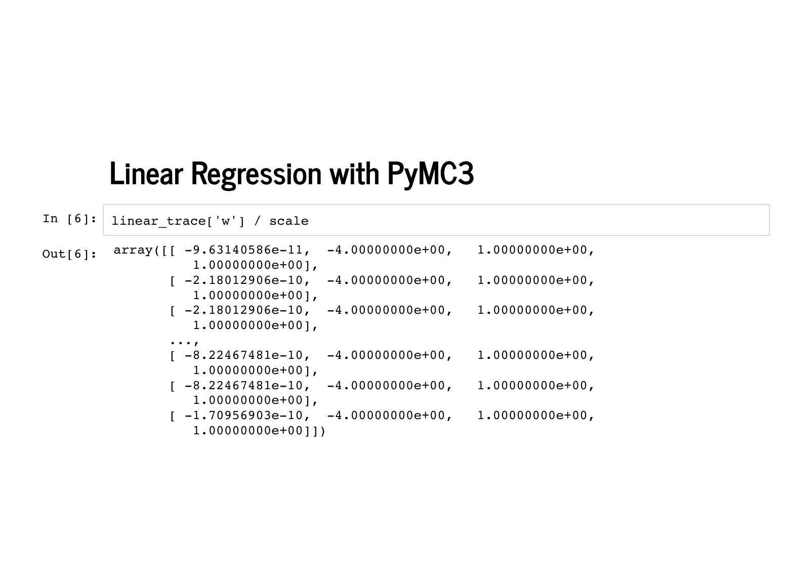
Inspecting the sampled weights, we see that every single sample was the exact right weights.

We are actually going to wrap the PyMC3 model inside a class with an sklearn interface, like we did earlier with the numpy model. We will just instantiate it with a function that eats a tuple X, y, and returns a PyMC3 model. Note that the predict method will be multiplying our data by a trace, so it will end up giving 2,000 plausible versions of our labels.

(Editor: Nicole Carlson gave a whole talk on turning PyMC3 into sklearn at the conference, and I recommend you catch the video)

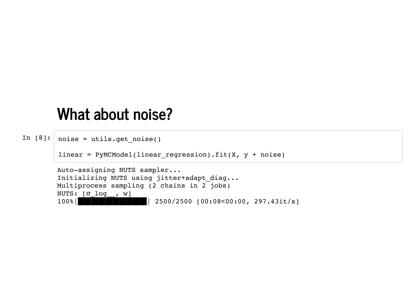
We can use this new class to fit the noisy version of our data. This takes a little longer, but we are not just sampling 2,000 copies of the same weights anymore.

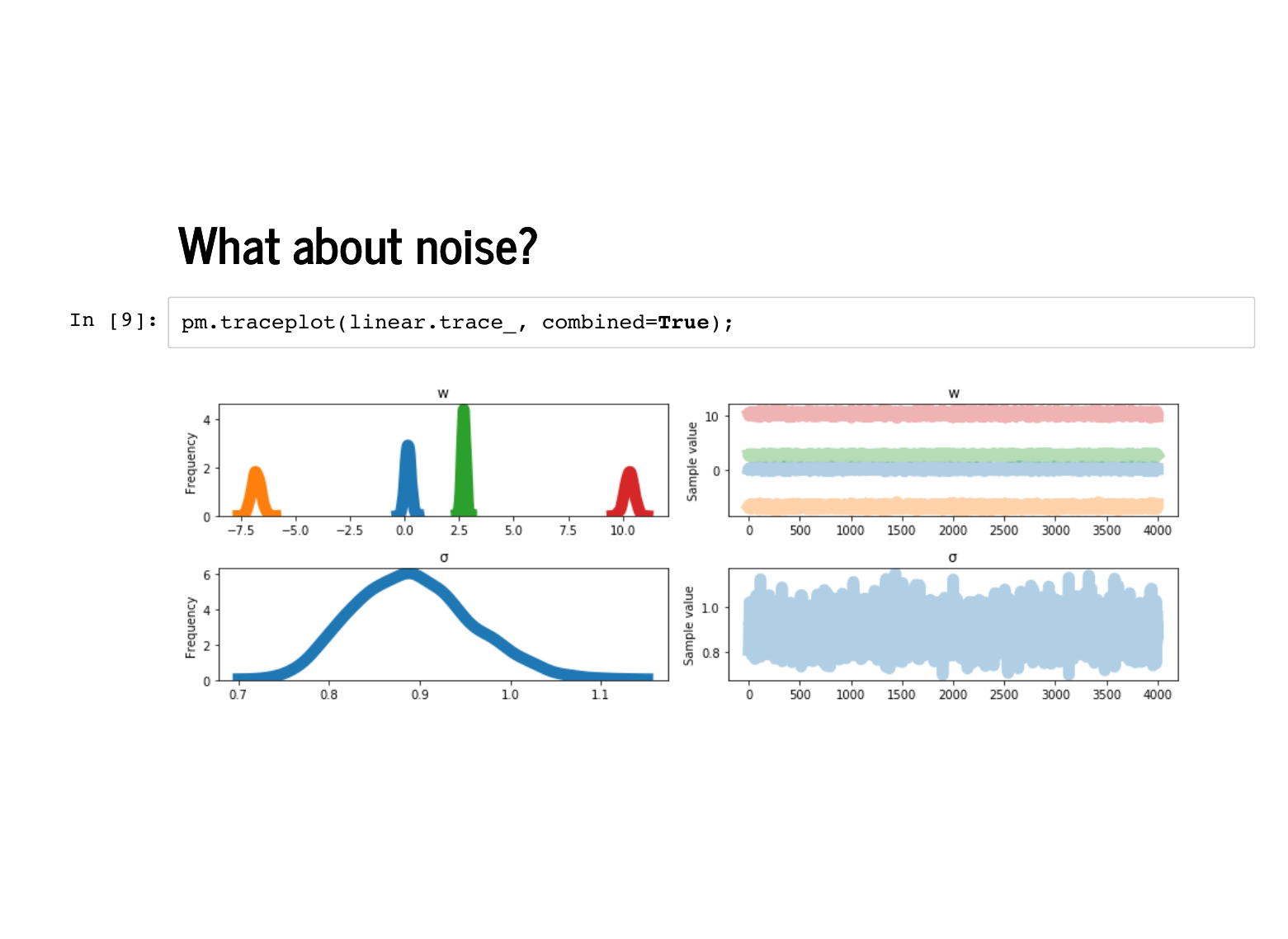
We can inspect the traceplot and see the weights are a little more dispersed, and the standard deviation is estimated to be somewhat less than 1.

The utils.plotter function actually has a few tricks up its sleeve. We plot 100 random sets of labels from the fitted model here, so that blue line is actually many lines. It is a pretty confident fit, so it does not disperse very much!

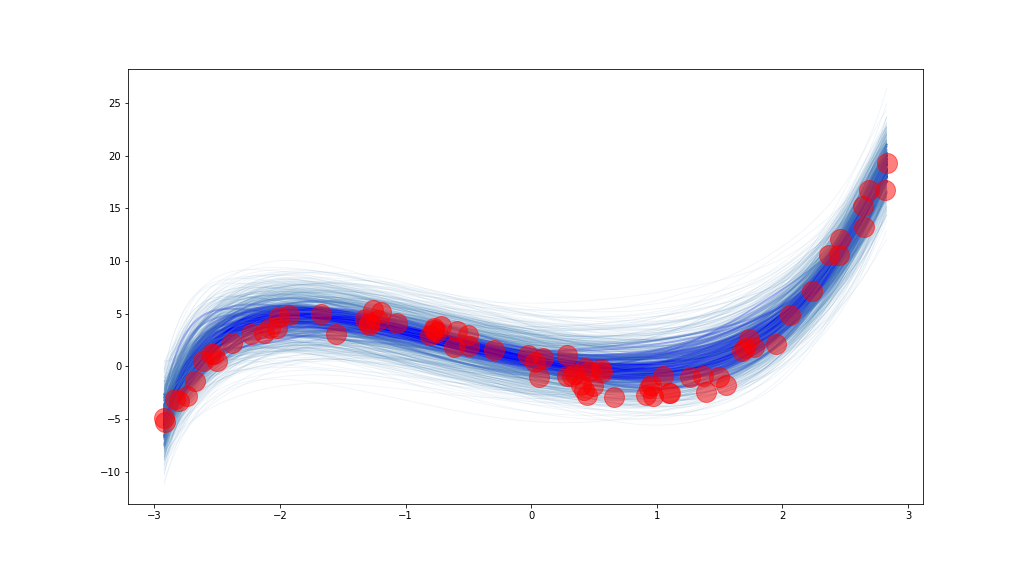
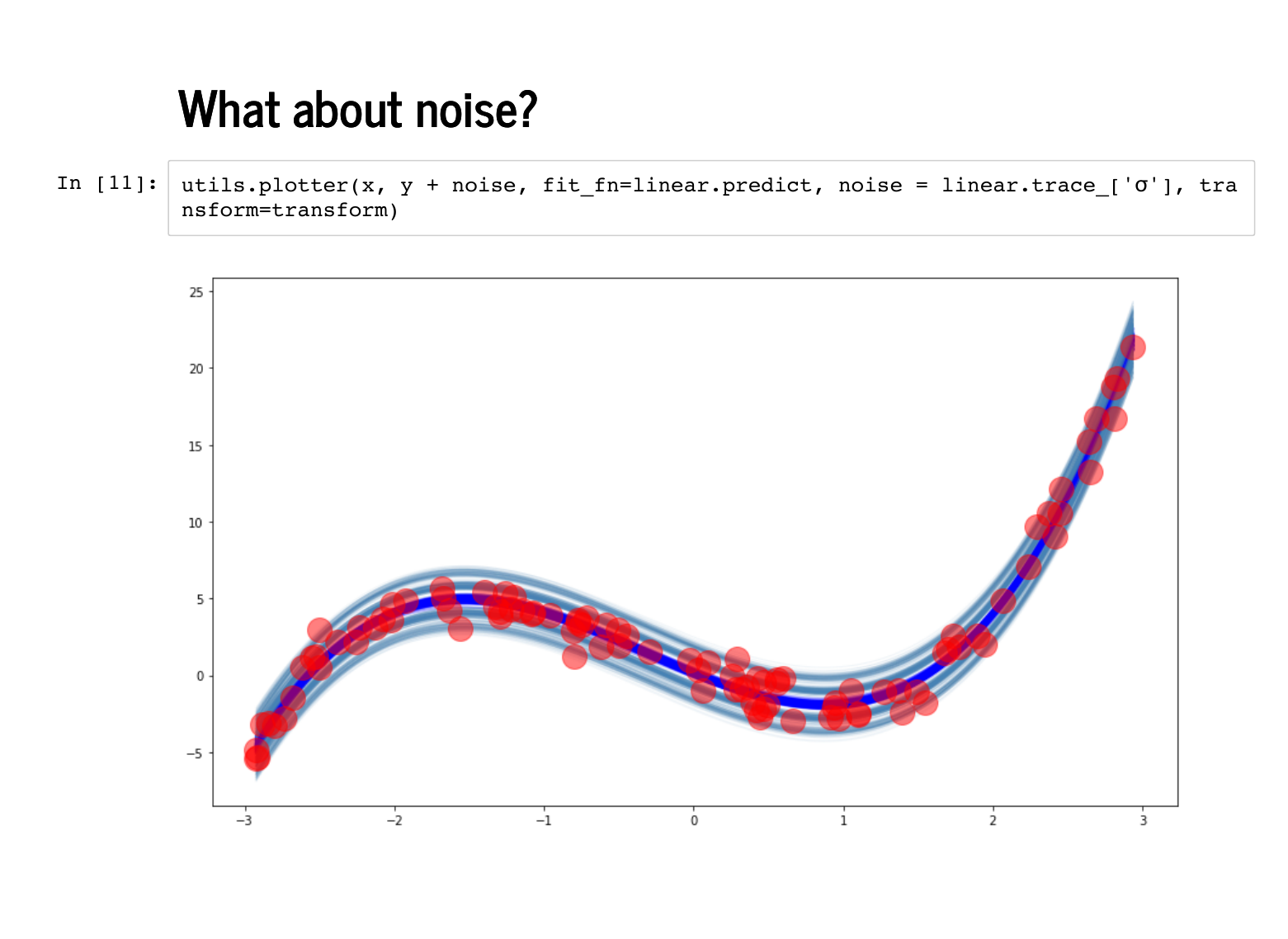
Remember that we also sampled the standard deviation. It is helpful to remember that we are sampling from a joint probability distribution, so each set of weights comes with its own sampled standard deviation. We plot here are 100 sets of weights, along with *their* standard deviations. There is a line at 1 standard deviation, and another at 2 standard deviations.

We knew a lot about modelling this data, so the fit looks almost too good. We will look at these plots again in a bad model later. For now observe that only one or two of the 100 points lies outside the second standard deviation line.

Exercise 6 is some practice at working with traces from a linear regression trace, and verifying that the right proportion of the data is 1 standard deviation off. Solutions are available here.

Now the takeaway from this last bit of the talk is that when we are regularizing, we are just putting a prior on our weights. When this happens in sklearn, the prior is implicit: a penalty expressing an idea of what our best model looks like. When this happens in a Bayesian context like PyMC3, the prior is explicit, expresses our beliefs about the weights, and can be principled.

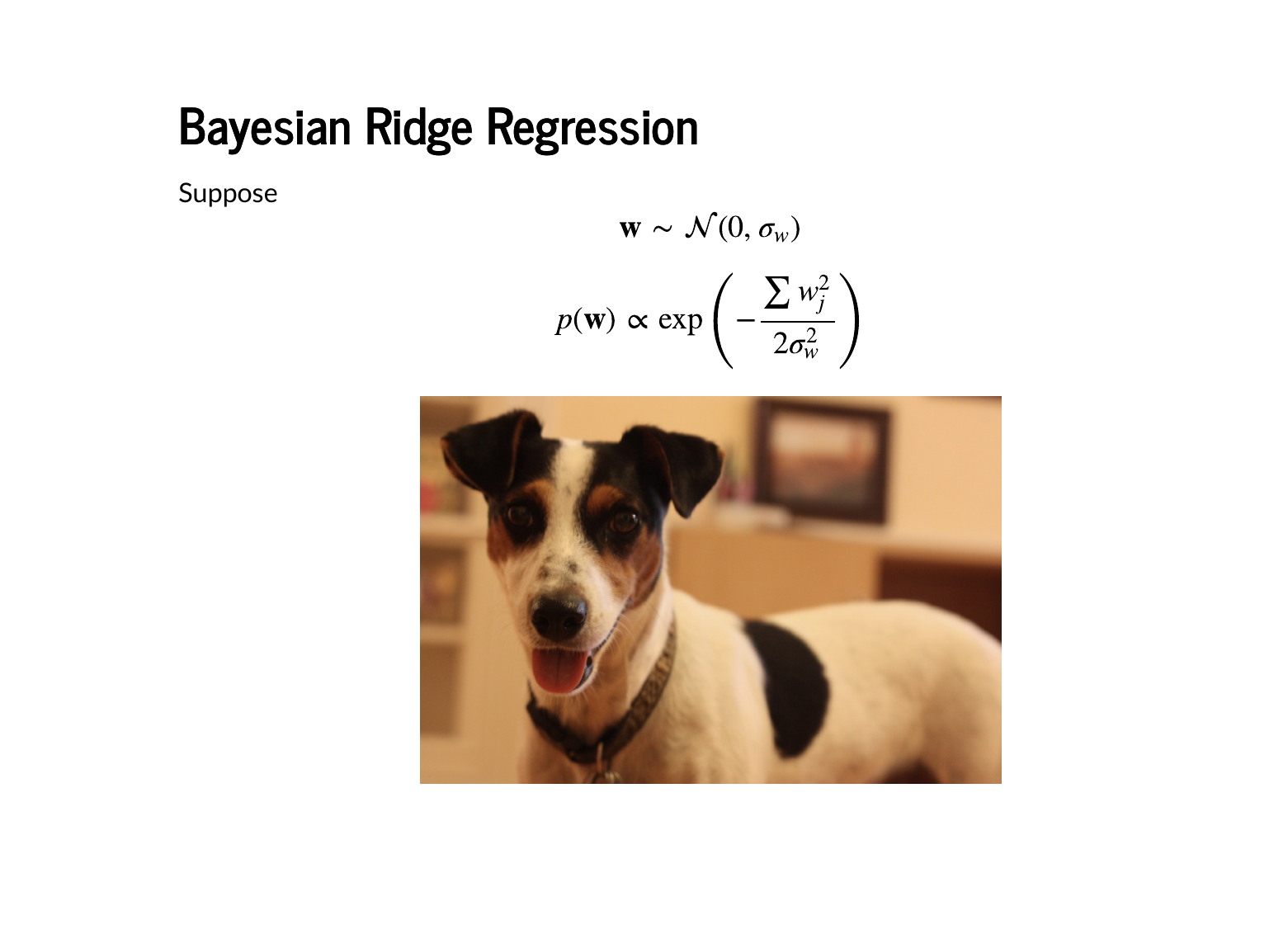
Ridge regression, for example, just means assuming our weights are normally distributed. Here is the pdf for a normal distribution again, this time centered at 0 with standard deviation σ_w.

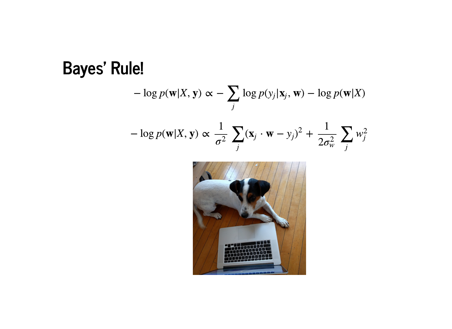
Recall that for any model, the negative log likelihood will be in this form: a likelihood minus a prior. We haven't change the likelihood, so it is still the sum of squared errors, but now our prior is the sum of the squared weights. Notice that this is proportional to the cost function from ridge regression in sklearn, so the maximum a posteriori estimate for this model is exactly the ridge regression weights.

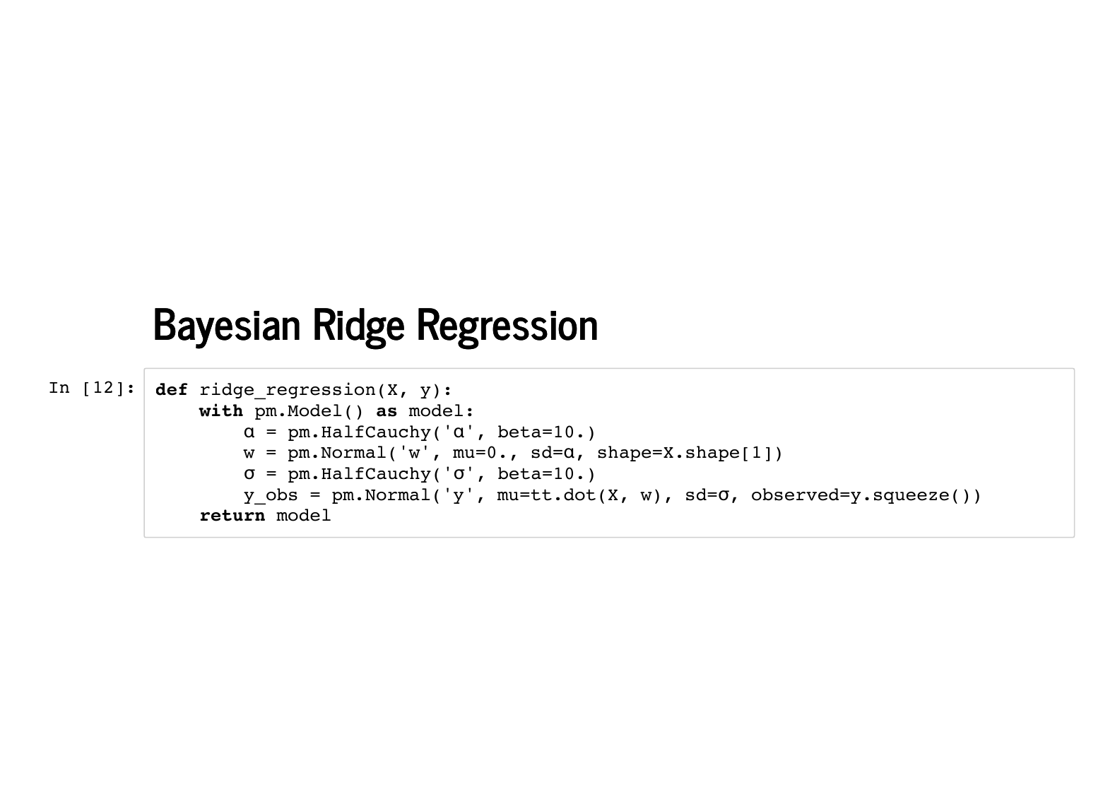
Here is that model implemented in Python. The differences from the first model are that we have changed w from a Flat distribution to a Normal distribution, and have added a term for the scale of the weights.

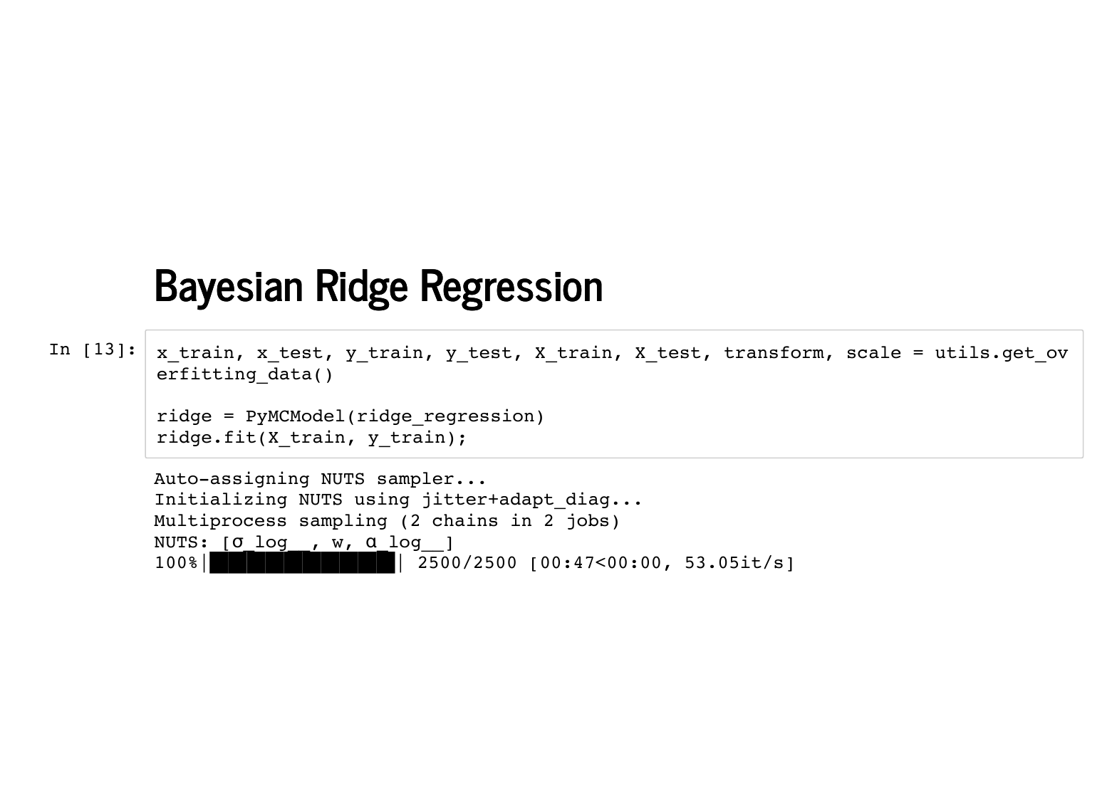
We can try the ridge model on the overfitting data from earlier along with our handy model class.

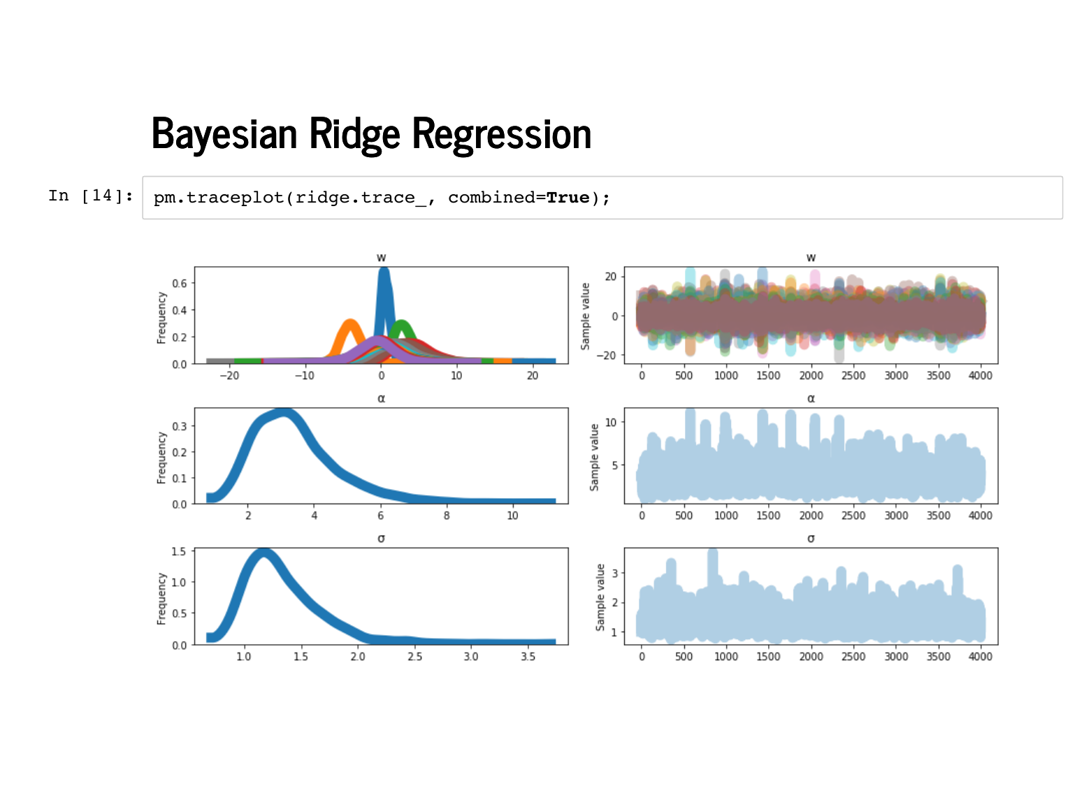
The trace plot gets hard to read with so many w's – there are fifteen now, remember – but there is nothing glaringly wrong in this plot.

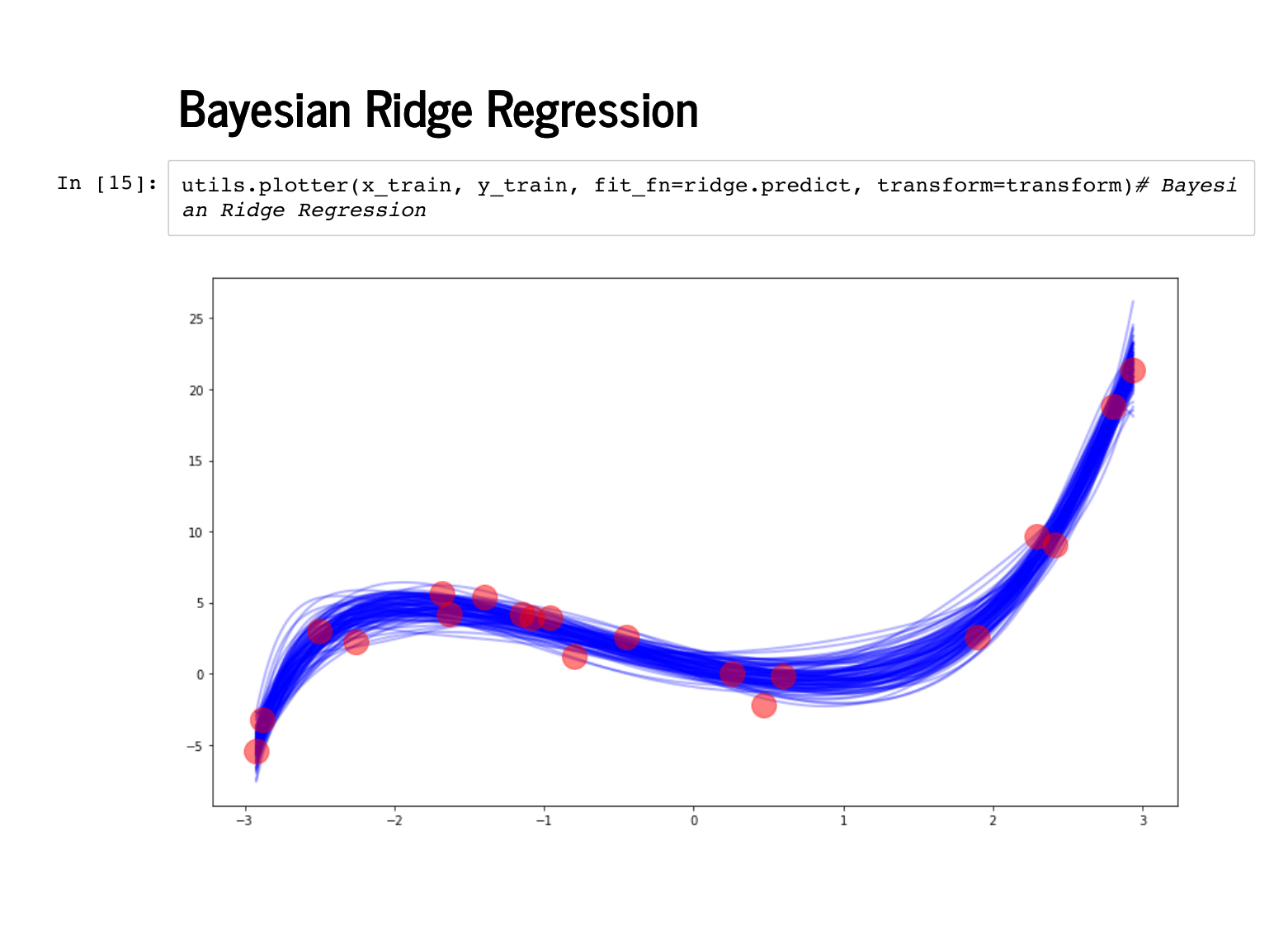
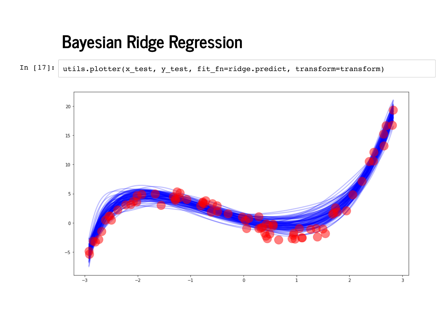
Here are 100 of our predictions on the training data.

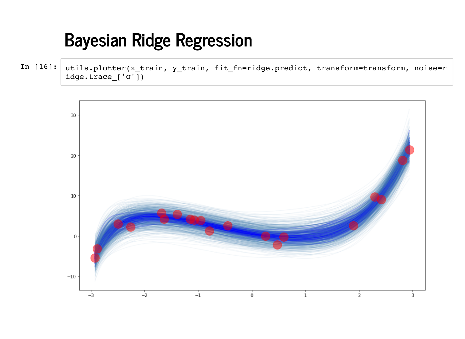
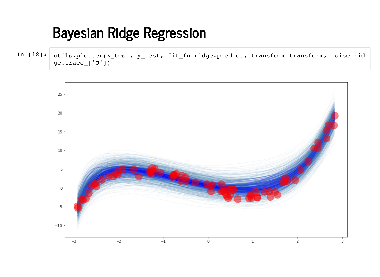
And here are the predictions along with lines for the standard deviation estimates.

It looks worse when we plot against the test data instead.

But the error estimates actually end up capturing a lot of the uncertainty properly here, particularly around x = 1.

Exercise 7 has you essentially derive the rest of the talk yourself. Check out solutions here.

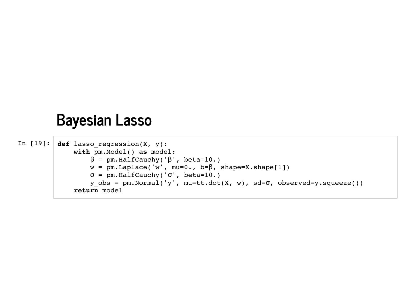
Remember putting a prior that looked like e^-∑w_j2 on the weights gave us ridge regression. It is quick to show that putting a prior that looks like e^-∑|w_j| gives us Lasso regression as a maximum a posteriori estimate. That particular distribution (once we normalize it) is the Laplace disribution, and it is built into PyMC3.

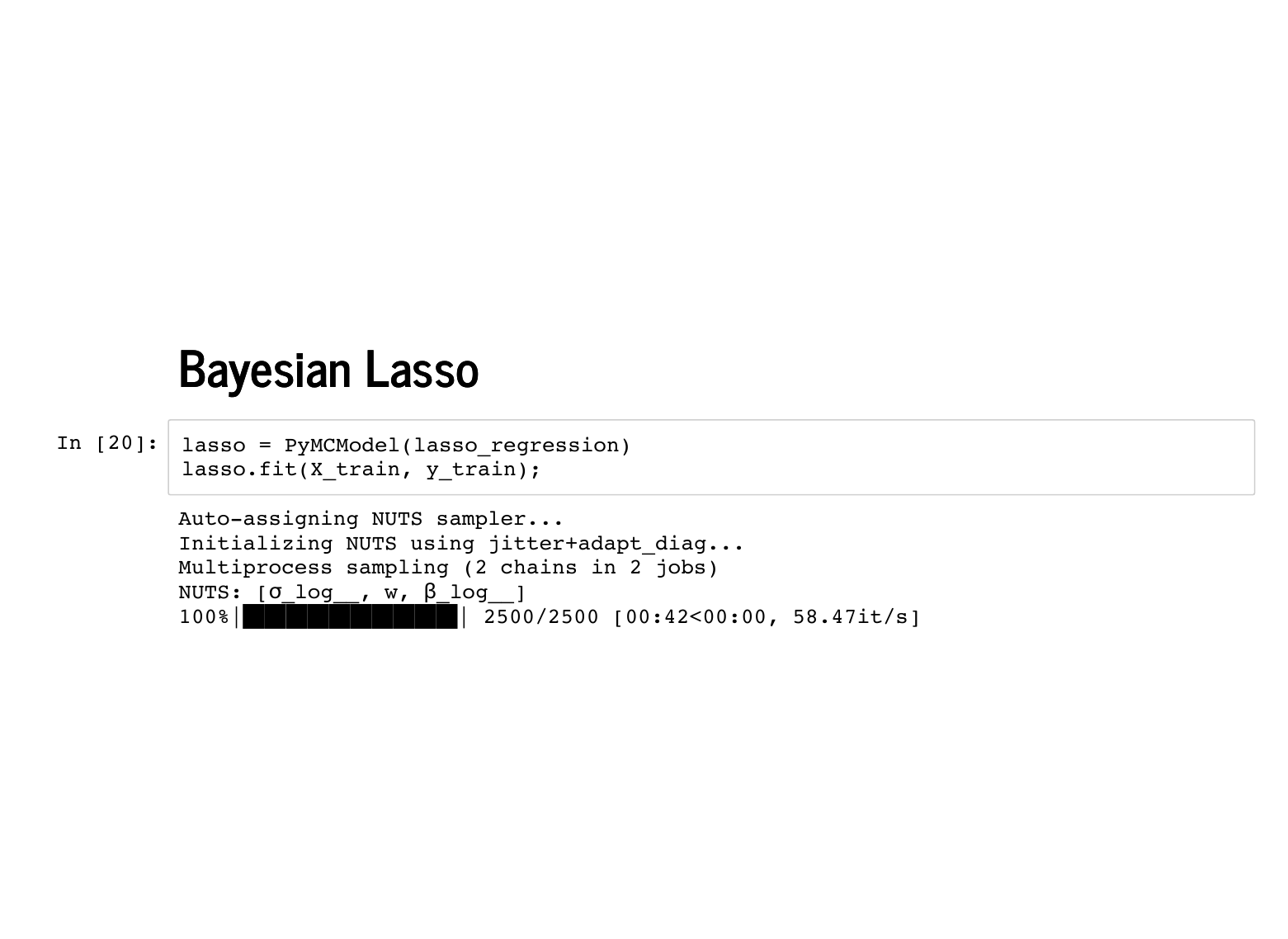
We have seen the rest of this talk already: first, we sample from our model.

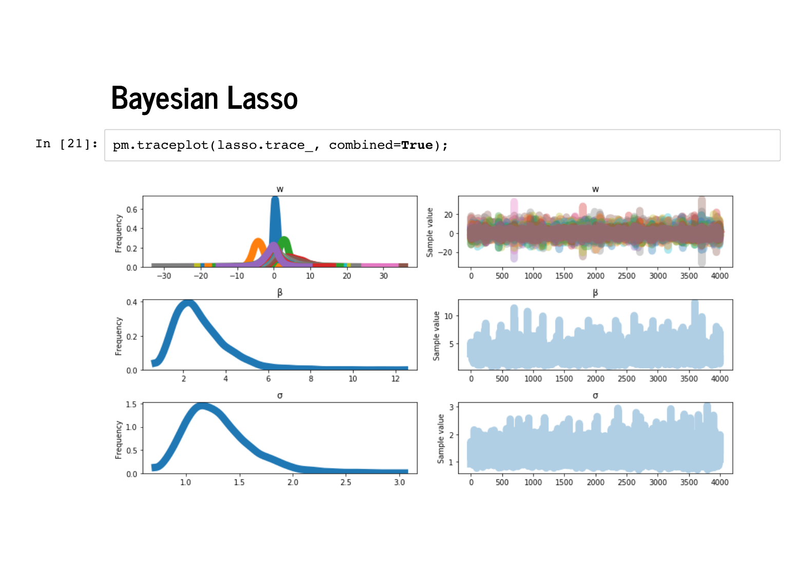
The traceplot looks fine, but always reasonable to check it out.

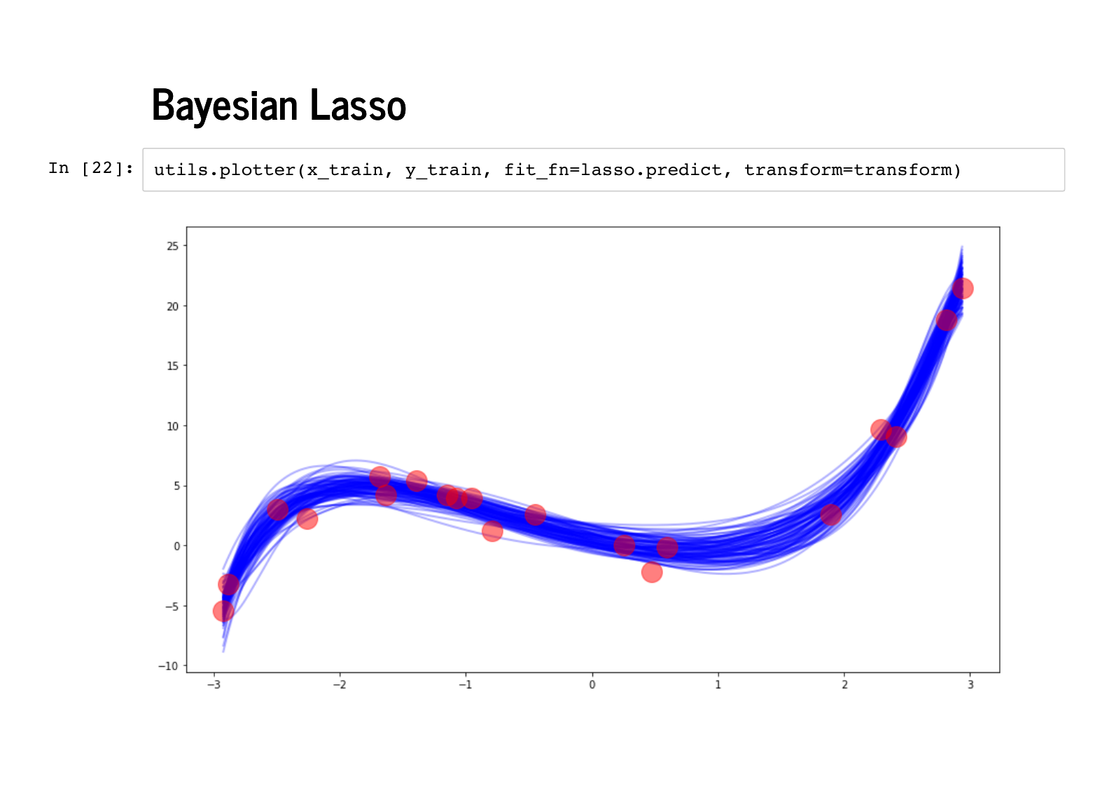
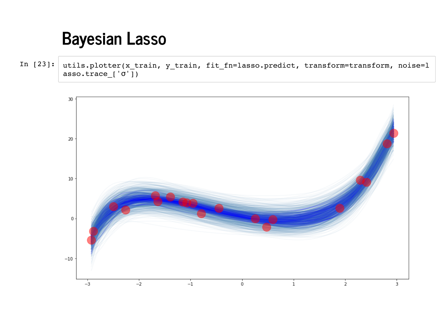
Now we can check out those spaghetti plots! First we plot against the training data, just for sanity.

These first two are good – remember that the fainter, greyer lines are the standard errors, and remember that we should expect our fit to be better on this data, since the model has already seen this training data.

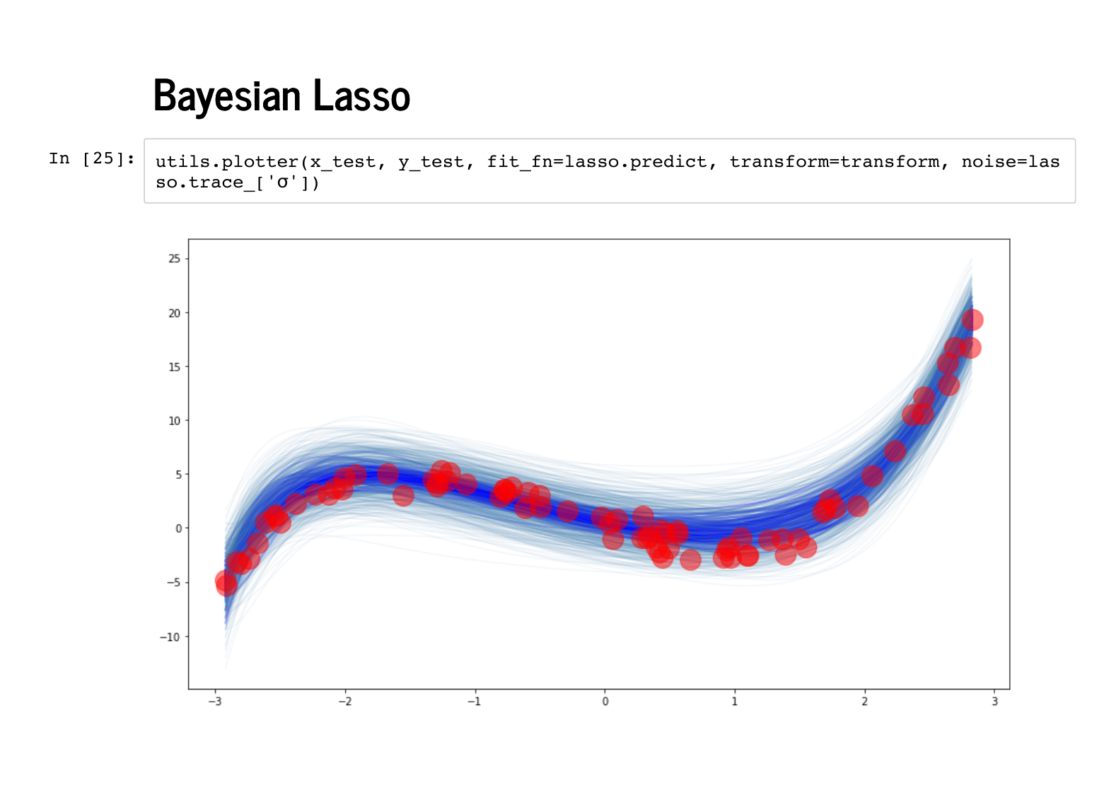
Now when we plot against the test data the fit still looks pretty good.

I want to conclude with a warning that the Bayesian ridge and Bayesian Lasso we talked about here are not models you should actually use. These were presented to show that you could recover scikit-learn models from a Bayesian model, and that you were secretly making some assumptions when you used these models.

In practice, what is to be done? We live in a Bayesian world, and you should model your weights using prior information you have about them. If you wish to model sparsity in your weights, Aki Vehtari and Juho Piironen have a recent paper proposing a better prior for a Bayesian treatment of sparse weights, and does a good job summarizing prior work on the topic.

It is a flexible world, and we should celebrate that. Thank you for coming.