
Hamiltonian Monte Carlo in PyMC3
These are the slides and lightly edited, modestly annotated speaker notes from a talk given at the Boston Bayesians meetup on June 15, 2017. Apologies to Maciej Cegłowski for ripping off the formatting of this essay.
There are a number of code snippets, figures, and demos that are in the talk. They are available to view or to download from the github repo. If you would like to run the code, you should have jupyter, and install the talk code with:
git clone git@github.com:ColCarroll/hamiltonian_monte_carlo_talk.gitcd hamiltonian_monte_carlo_talkpip install -r requirements.txtjupyter notebook
The code was run using Python 3.6.1, but will probably work with any version. Feel free to suggest corrections via github, get in touch on twitter, or see other projects on my personal site.

|
Thank you all for coming. I am Colin Carroll. I am currently a software engineer doing natural language processing at Kensho, where we are hiring, and in my previous life I was a pure mathematician. When my parents ask me what the "pure" in "pure mathematics" means, I tell them that I did not use a computer. Since then I have been using a computer pretty constantly, and hopefully in this talk you will see some sort of mix between that theory and practice. |
|
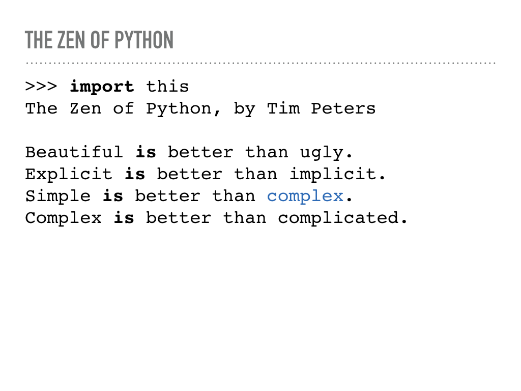
Today I am talking about doing Bayesian inference using Python. It is a wonderful language to work in, it is expressive and beautiful, but at the same time, allows us to call out to more powerful languages for speed. More importantly, but certainly related, there is a rich ecosystem of libraries for Python that we can use and build on top of. I will actually be using a small library I built wrapping PyMC3 called |
|
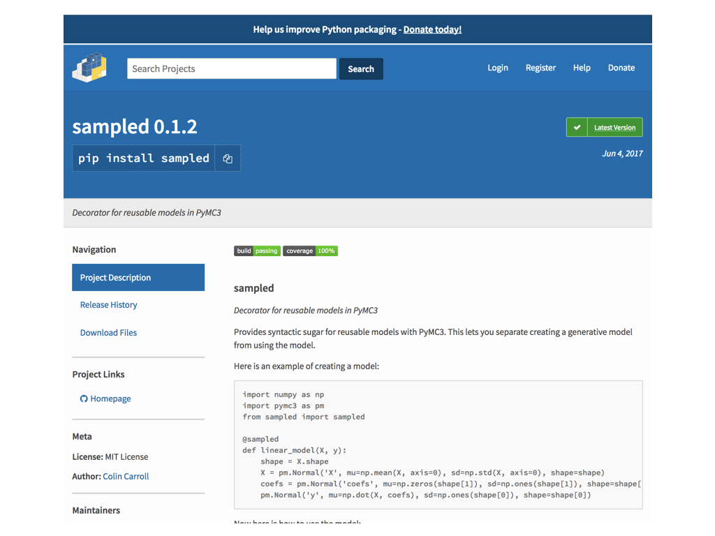
As a brief diversion into open source, this is a beautiful thing: if a library does not do what you want, you can often fix it and share it back with the maintainers. Or, if you just want to be able to install your doubtless brilliant work on any computer, there is free infrastructure out there to help you share what you built back with the world. As an example of the latter, I will emphasize here that As an example of the former, I got involved with PyMC3 about a year ago when I got annoyed by their test suite during my long train commute. You know it gets when someone is wrong on the internet. Since then, I have used working on the library as an excuse to learn more about Bayesian inference. I think it is a welcoming community, we are always looking for new contributors, and I am happy to talk more about getting involved in open source. I know I was interested for a long time, but it is difficult to know how to make the first step. We even have stickers! |
|
|
|

|
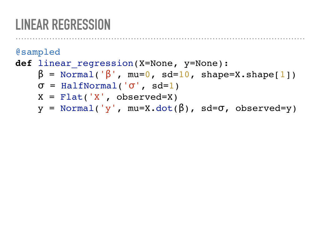
As an example of the expressiveness of Python, and a review of how Bayesian inference might be useful, consider this definition of Bayesian linear regression from Wikipedia. We are supposing we get a matrix of observations X, a vector of labels y, and we’ll try to recover the weights ß and noise σ. This being a Bayesian treatment, we will expect to get a(n estimate for the) full posterior distribution for these variables. |
|
Here is the exact same model written using PyMC3 and |
|
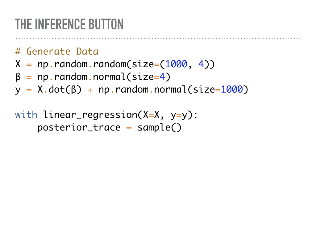
How do we use this model? We can give it some artificially generated data and let PyMC3 sample from the posterior. This is done in the Note that the context manager |
|
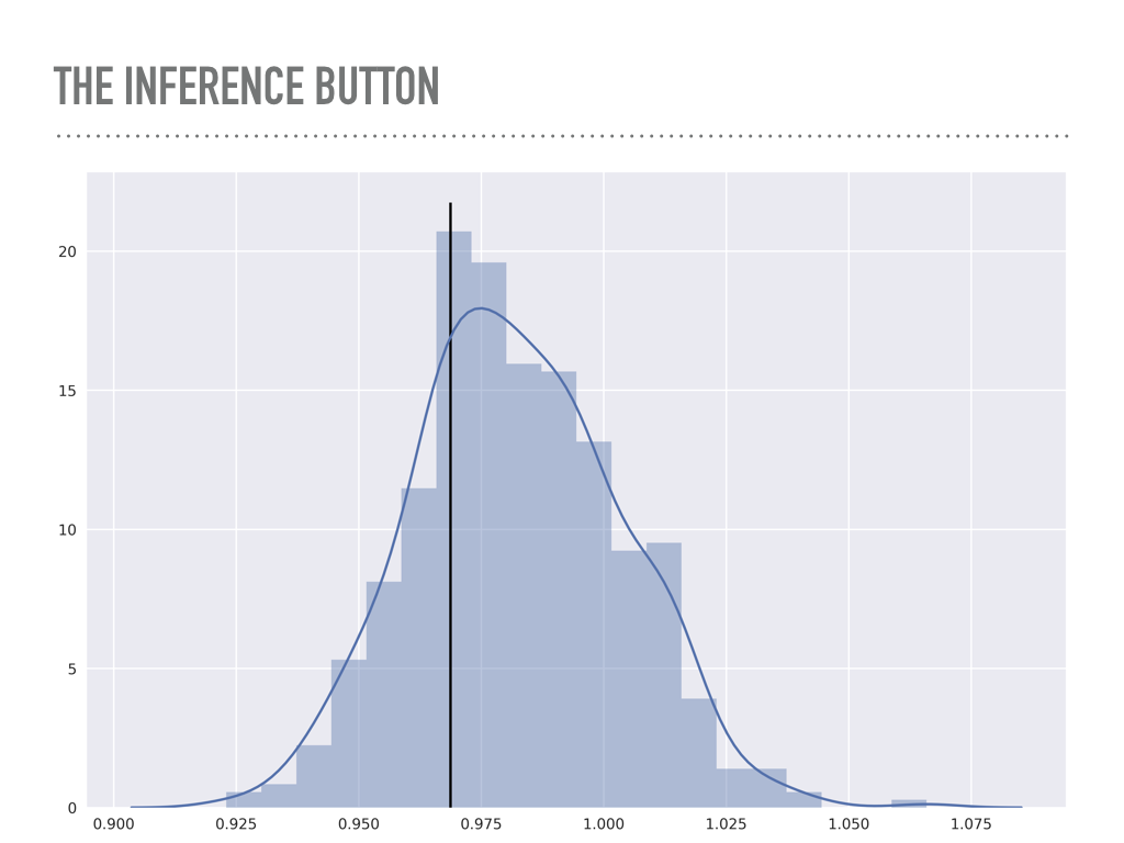
Here is a plot of 500 points from the posterior distribution of the noise variable σ. The true value is marked with the solid line, and you can see I added quite a bit of noise for this model. |
|
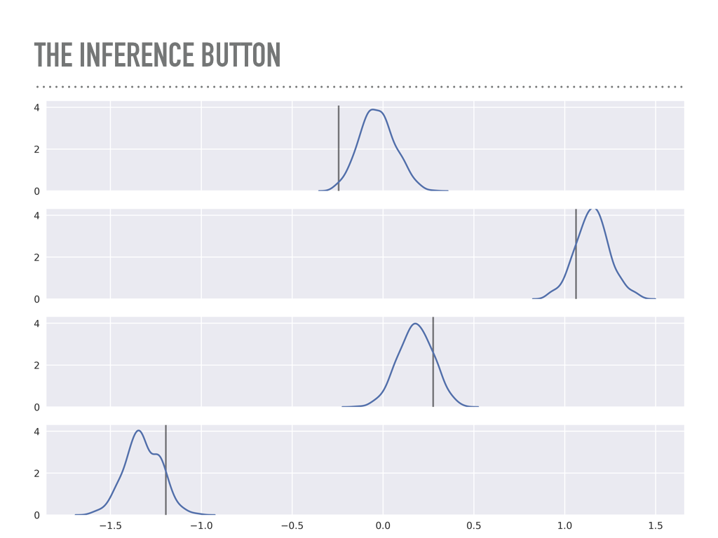
These are the posteriors of the weights ß that were sampled. You can inspect either the plot or the actual traces and confirm a really calming fact: math works, which is great: the maximum of each of these distributions is quite close to the maximum likelihood estimator you would get from minimizing least squares, or fitting this data with scikit-learn. This continues to impress me, that this apparently very different algorithm from statistics can recover the same point estimate as linear algebra or calculus would. It is like a math trifecta. Notice that the maximum likelihood is not exactly the values we used to generate this data, but by using this approach, we may quantify how surprised we are at the true values. |
|
|
|
|
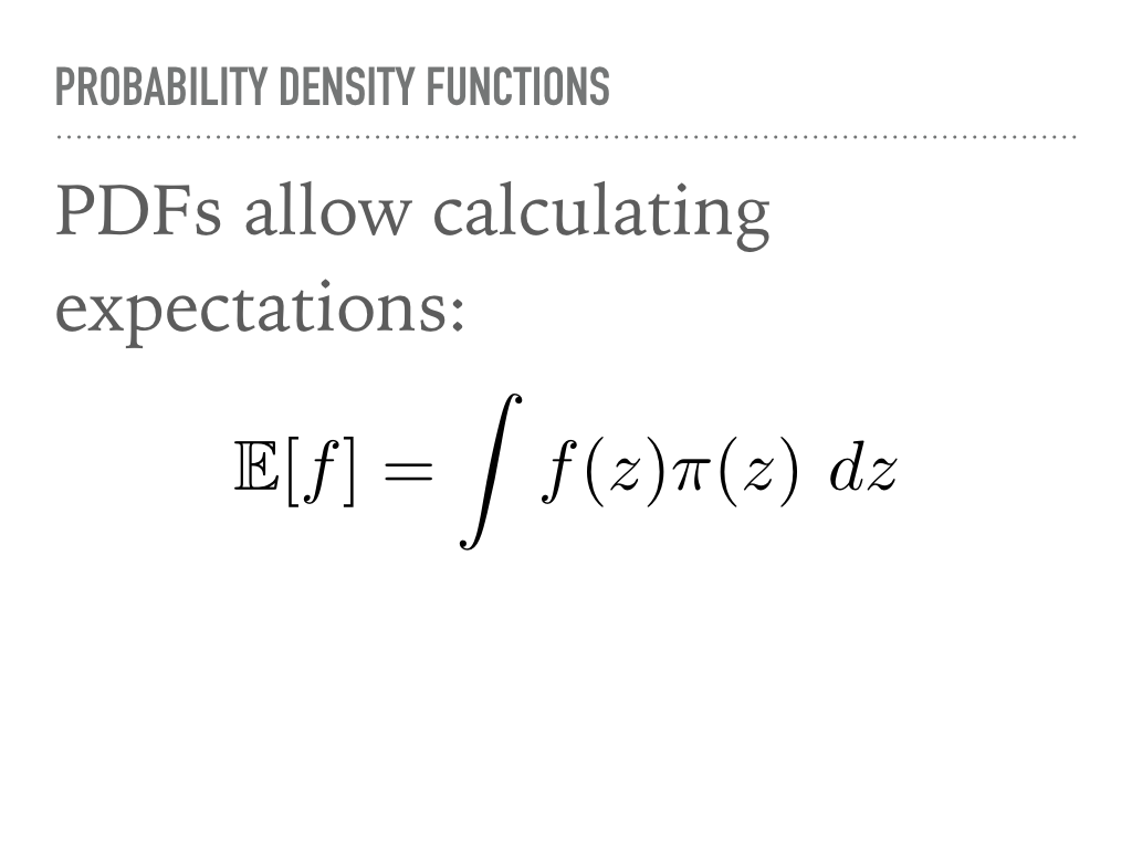
How does this sampling actually work? I am going to follow the approach from Christopher Bishop’s book Pattern Recognition and Machine Learning, as well as borrow quite a bit from Michael Betancourt, particularly when discussing Hamiltonian Monte Carlo. There are links to sources at the end of the talk. As a brief review, a probability density function is a way of assigning probability to an event. In the case of discrete events, this is quite intuitive, and a often a question in combinatorics involving urns, dice, birthdays, and marbles. In grad school I studied measure theory, and in the language of that field, a pdf assigns measures to sets. In general, a measure - and hence, a pdf - only makes sense under an integral sign. So to emphasize a point we will return to, we care about sampling from probability density functions because we care about calculating expectations. |
|
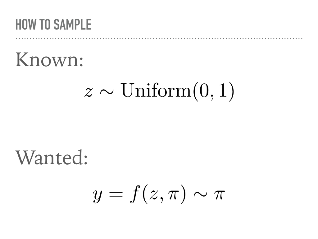
As a first, fairly classical approach to this problem, we suppose we are able to generate uniform random samples. How that happens is beyond the scope of the talk, but we will trust the We also suppose we have a pdf π, which we can evaluate at points: think of the Gaussian where it is easy enough to write down the function. More generally, and we might think of π as being the posterior of some big joint probability distribution in the presence of data. Evaluating the posterior distribution at points is still easy because of Bayes’ Theorem. The goal is to generate samples distributed according to π using only our uniform random number generator and this knowledge of the pdf. |
|
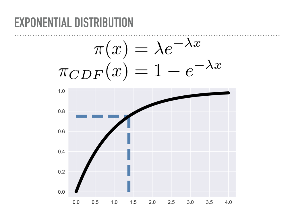
A natural way to do this is to invert the cumulative density function. Here we have the pdf for the exponential distribution, and have plotted the cdf. When we draw 0.75 from our uniform distribution on the y-axis, we will walk out horizontally until we meet the cdf, then see the x value that corresponds to — here, something like 1.4 |
|
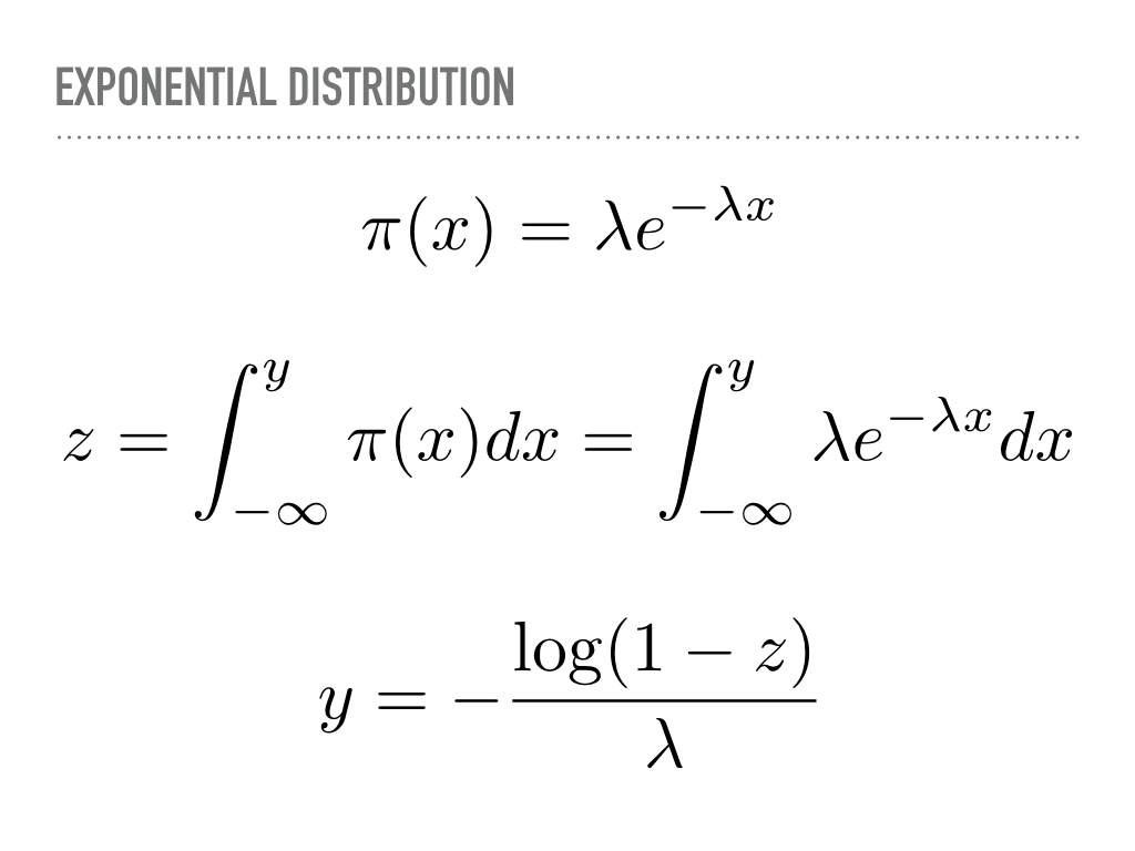
Here is what we just did analytically. Just let your eyes soak that in. Somewhere in there, we are evaluating an indefinite integral, and then inverting it with respect to one of its limits. For the exponential distribution, this is tractable, so we may sample from that distribution nearly as fast as we sample from the uniform distribution. |
|
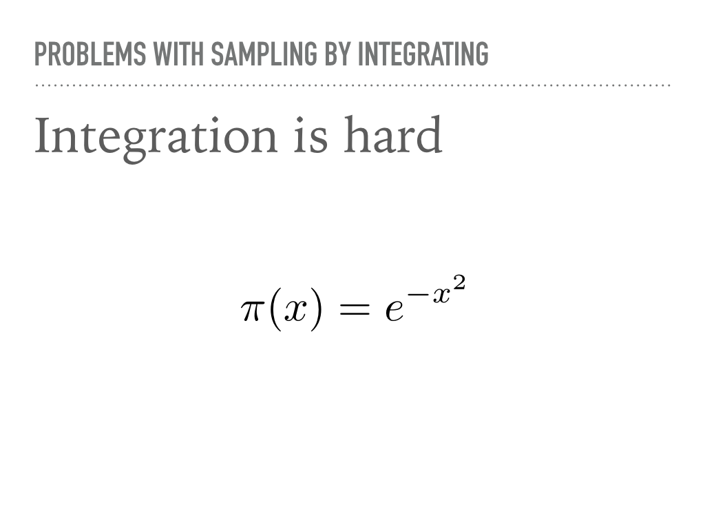
However, in general, integrating is difficult. The Gaussian pdf is famously non-elementary. There happens to be a trick for generating two i.i.d. normal numbers from two uniformly distributed random numbers, but it is untenable to expect integration to work all, or even most of the time. However, note that we now have some distributions that we are able to sample from besides the uniform one. In particular, you should expect “named” distributions will have a fast sampling method. Our goal then is to sample from more complicated distributions, where it is not reasonable to hand craft an integration scheme whenever the model changes. |
|
|
|
|
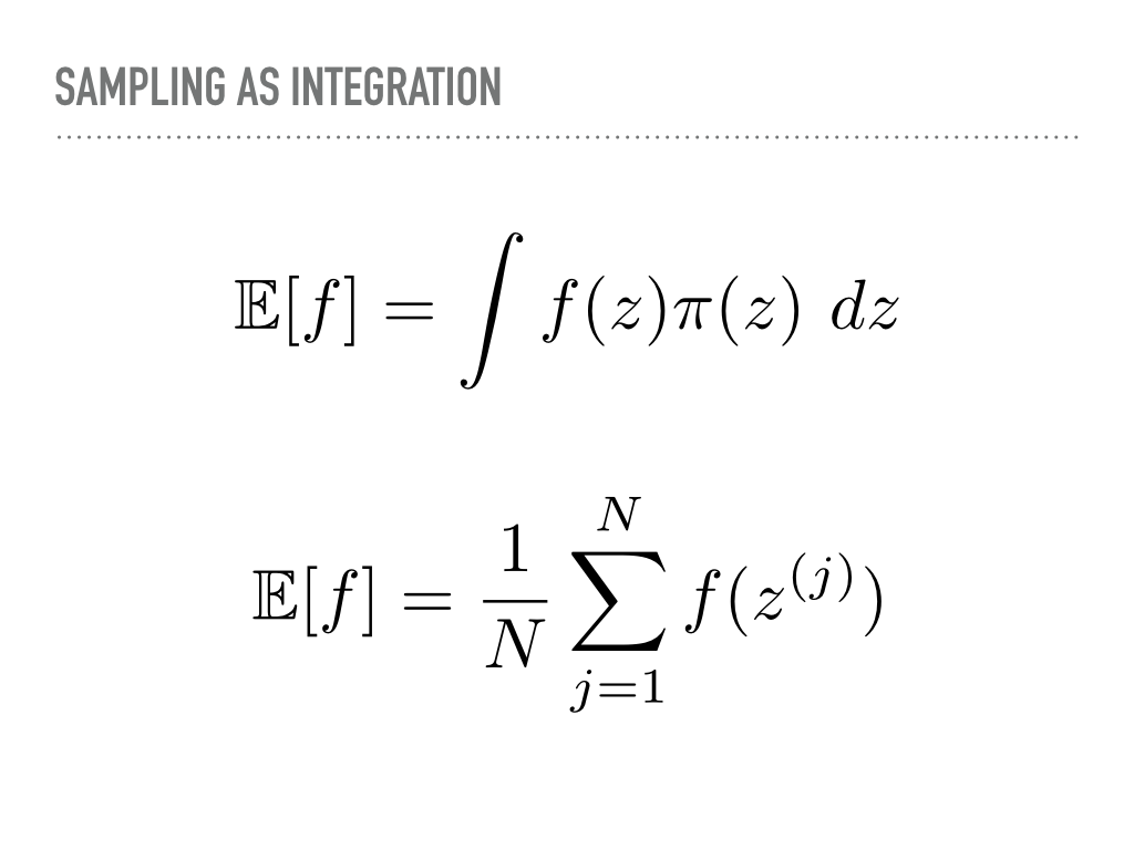
In light of this desire for a more general way of evaluating integrals, let us re-examine our strategy. We are interested in computing expectations, and to do so, we will pass from considering a continuous integral to an approximation of it using discrete samples. Specifically, we will sample a sequence of variables z(j) from our target distribution π, and average the value of the function over those points to compute our expectations. |
|
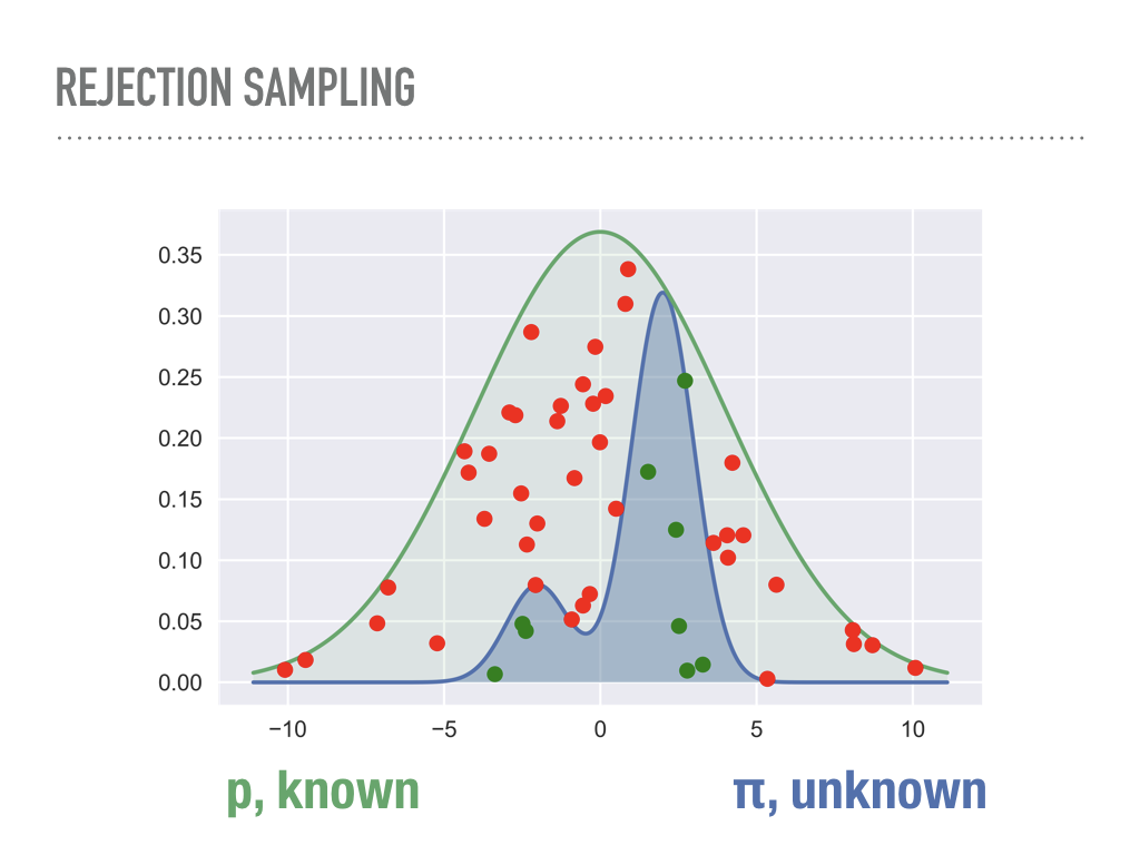
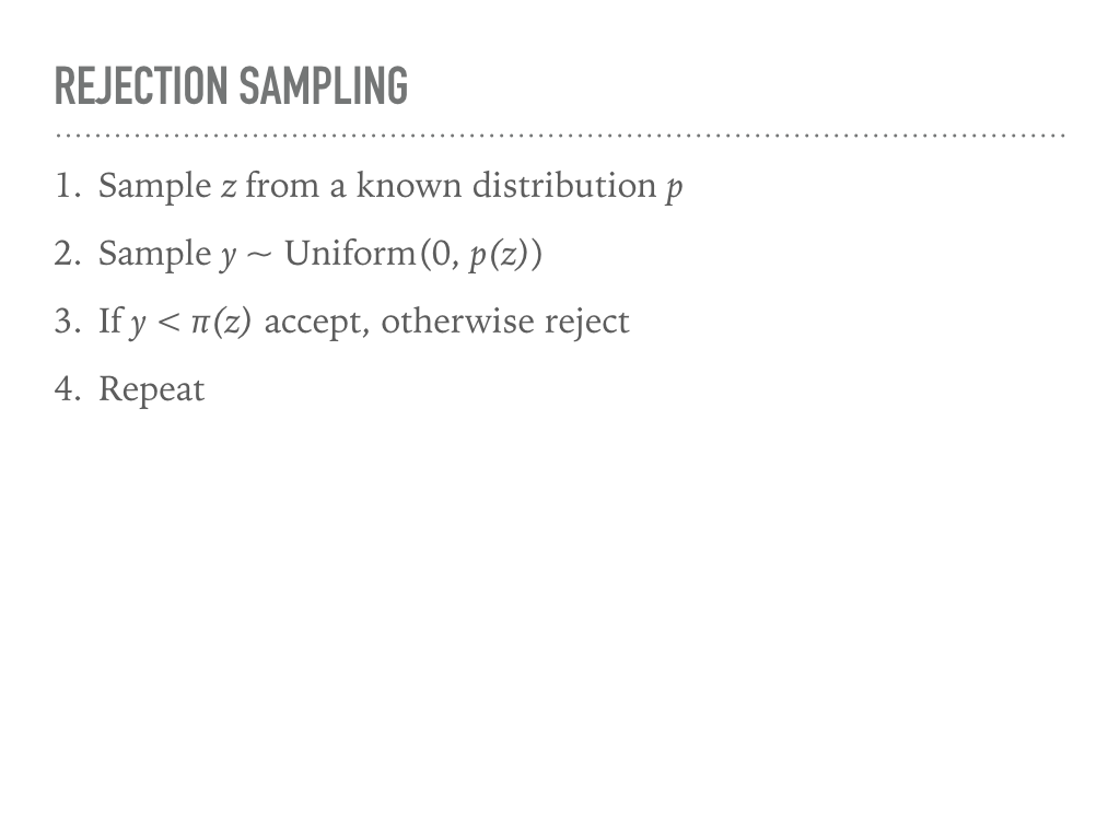
Our first attempt at a general approach is called rejection sampling. The algorithm is simple, but the picture of what is going on is even simpler. We choose a known distribution p and scale it so it is always larger than the distribution of interest, π. Here we have chosen a scaled normal distribution. We sample repeatedly and uniformly from underneath p, and accept any samples that are also under our unknown distribution. This sampling is in two steps: first we get a sample along the x-axis from p, then a uniform sample between 0 and p(x), which we compare to π(x). It is not hard to show that the green points end up being independent samples from π. The red points are the computational cost we pay to do rejection sampling: the closer our proposal distribution matches our unknown distribution, the less computationally expensive generating random samples is. But that is also one of the problems with rejection sampling. |
|
Intuitively, we are sampling from a uniform distribution underneath one curve in order to measure the area under another curve. This known distribution p has to be bigger everywhere than the unknown distribution, but we are not even using the fact that the it is a probability density function here, only that we can sample from it. |
|
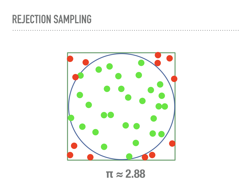
A problem with rejection sampling is that it is still not really “general”, in that we must design a proposal distribution that dominates our unknown distribution. The worse our proposal, the more computational time we are wasting as we reject more samples. In higher dimensions, this problem is compounded. To understand this, consider a common method of approximating the area of a unit ciricle by sampling points from the square with side length 2, and accepting those samples that are within the circle. Note that this is secretly approximating the uniform distribution on the unit circle using rejection sampling. This will converge, if a little slowly. In a few seconds my laptop had a passable approximation for π (the constant, not the distribution). |
|
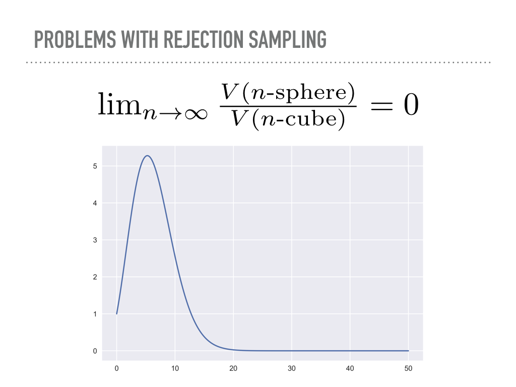
But suppose now we wanted to sample the unit n-sphere, and use the enclosing hypercube as the proposal “distribution”. In n-dimensions, this cube has volume 2n, while the volume of a hypersphere converges to zero. This is an unintuitive fact, that all of the volume in a high dimensional cube is in the corners, that should also serve as a warning that our geometric hunches may not be accurate in high dimensions. I did not actually believe the math here was as bad as all that, and tried this with numpy. In a recurring theme today, math works, and in ten million samples from a twenty dimensional cube, none of them were inside the unit hypersphere. |
|
|
|

|
There are various partial fixes to rejection sampling, and you can actually sample pretty effectively by hand-tuning a proposal distribution, but it seems hopeless to build an efficient “inference button” this way. In searching for a general sampling method, we turn to Markov Chain Monte Carlo. A Markov chain is a discrete process where each step has knowledge of the previous step. Markov chains are useful in sampling because, in distributions of interest, regions of high probability tend to “clump”, so once your chain finds a region of high density, it should stay in a region of high density. We will discuss this more later in the context of “concentration of measure”. |

|
This is my dog Pete, exhibiting how a Markov chain might explore a region of high scent density (click through for gif). He wanders off briefly in the middle, but then goes back to the good stuff. This is roughly how Metropolis-Hastings works. If he was good at following scents, I might have another video of him demonstrating Hamiltonian Monte Carlo, but he does not want to go too far from the good stuff. |
|
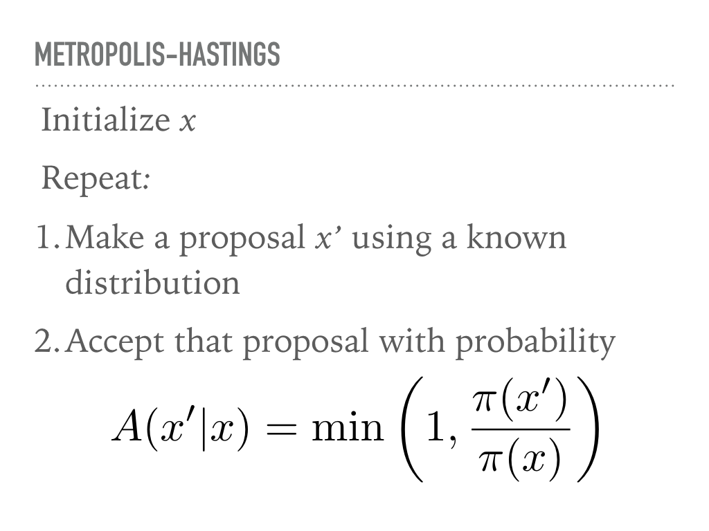
This is a cartoon of how Metropolis Hastings sampling works. Suppose we have a two dimensional probability distribution, where the pdf is like a donut: there is a ring of high likelihood at radius 1, and it decays like a Gaussian around that. Metropolis-Hastings is a two step process of making proposals, and then deciding whether or not to accept that proposal. When we reject a proposal, we add the current point back to our samples again. This acceptance step does the mathematical bookkeeping to make sure that, in the limit, we are sampling from the correct distribution. Notice this is a Markov chain, because our proposal will depend on our current position, but not on our whole history. |
|
For more rigorous approach, we can look at the actual algorithm. You can see the two steps here: first, propose a point, then accept or reject that point. This acceptance step makes those two steps work together just right and we will actually be sampling from π in the limit. We will again start with a proposal distribution, but this time it is conditioned on the current point, and suggests a place to move to. A common choice is a normal distribution, centered at your current point with some fixed step size. We then accept or reject that choice, based on the probability at the proposed point. Either way we get a new sample every iteration, though it is problematic if you have too many rejections or too many acceptances. There are some technical concerns when choosing your proposal, and the acceptance here is only for symmetric proposal distributions, though the more general rule is also very simple. But this is it, and this is a big selling point of Metropolis-Hastings: it is easy to implement, inspect, and reason about. Another thing to reflect on with this algorithm is that our samples will be correlated, in proportion to our step size. But I want to really emphasize that this bookkeeping is just beautiful in that it is the exact right thing to make sure our samples come from the correct distribution in the limit. This is a theorem with a fairly simple proof - see detailed balance. There are cases where the convergence is truly only at infinity, which continues to be difficult to automatically diagnose, but if we are using MCMC, we are no longer worried about if samples will converge, only when samples will converge. |
|
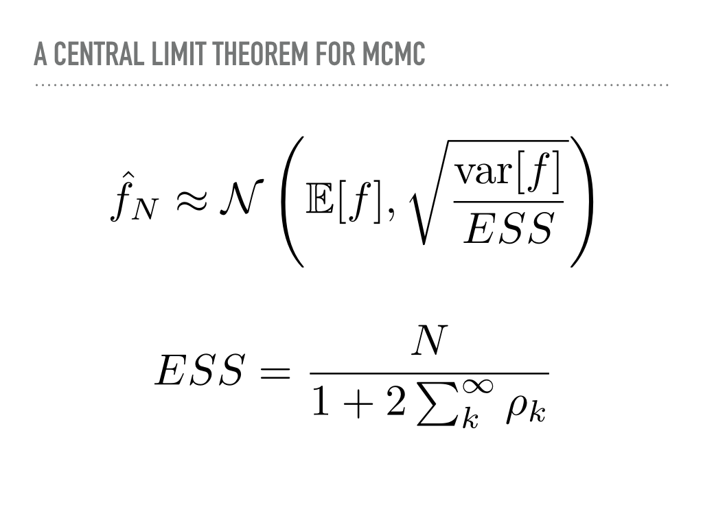
In fact, the central limit theorem for MCMC says that the sampled expectation will be normally distributed around the true expectation. ESS here is the "effective sample size". In the best case, the effective sample size is the number of samples, meaning each decimal place of accuracy will require one hundred times the number of samples. However, more correlated samples means a lower effective sample size, meaning more noise in our estimates. So you might have 1,000,000 samples, but the ESS is still only 10 because the draws are so correlated. This is something often reported in the PyMC3 issues, which is also a UI problem: we have a beautiful progress bar for sampling that tells you exactly how many samples you get per second, and this makes it obvious that Metropolis-Hastings gets far more iterations per second than more state of the art sampling methods. This is because iterations per second can be a poor proxy for the effective sample size, which is what is important. |
|
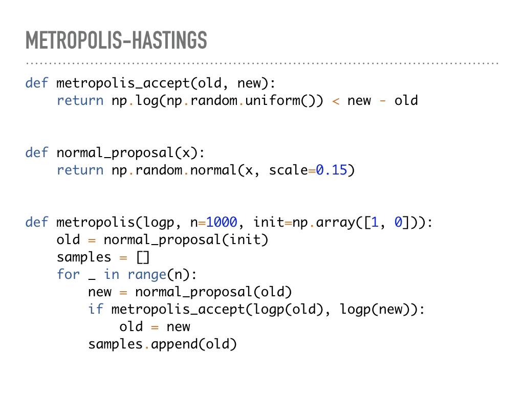
Here though is a full implementation of Metropolis-Hastings in Python. Notice there are a few knobs to turn, like the step size, the proposal distribution, and the initial point. There is some research that says 0.234 is the optimal acceptance rate for certain classes of distributions. By making the step size smaller, you can increase your acceptance rate by staying close to regions of high probability. Conversely, you can increase the step size, and make bolder proposals that get rejected more often. The price you pay in either direction is that your Markov chain will not explore space as quickly, and your samples will be correlated. For an initial point, Michael Betancourt makes a wonderful case for not using the maximum likelihood estimator: if you have a survey with 50 questions, no one will look like the average response to all those questions. You might prefer to use one of the people in your survey as a “representative sample”. PyMC3 will use a “tuning” period to automatically set both the initial points and the step size, optionally discarding those samples (when we change the proposal distribution, we lose our theoretical convergence guarantees). |
|
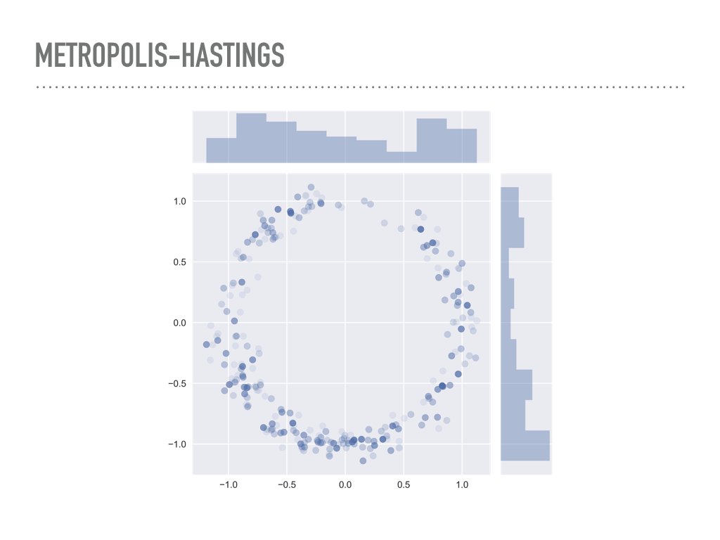
Here are 1,000 samples I took using the previous function from a “donut” distribution. The pdf is normally distributed about the unit circle, with standard deviation 0.1. There is some transparency to the points, and the darker ones are places where there were rejections before making the next jump. The actual acceptance rate of these samples was around the optimal rate. |
|
However, high dimensions plague Metropolis-Hastings too. We are constantly looking for the right step size that is big enough to explore the space, but small enough to not get rejected overly much. High dimensions has tons of space, and it gets harder and harder to stay in a region of high probability while also exploring the whole distribution at a reasonable rate. |
|
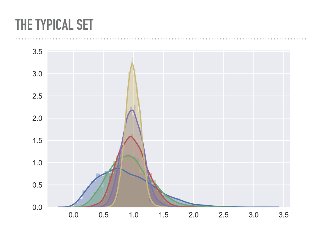
This is a plot of the average radius of points drawn from multivariate Gaussians in increasing dimensions. Notice how the points start to concentrate in a band — blue is one dimension, green is two, and so on. In this case you can imagine yellow represents a 6 dimensional “shell” that is distance 1 away from the origin, and this is common in high dimensions: in a rigorous way, there will be an exponentially small area where a pdf is big. This is problematic because no matter how well we tune Metropolis-Hastings, it will be too computationally expensive to explore the entire probability distribution. It is a fine choice for low dimensions, but once your model has more than a few dimensions, convergence may be quite bad. |
|
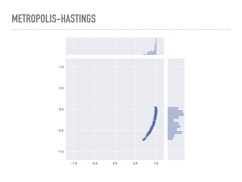
You can actually see this in low dimensions by making the derivative of the pdf large. Here are samples from the donut distribution again, but instead of having a standard deviation of 0.1, we use a standard deviation of 0.01. You can see that 1000 samples was not nearly enough to explore the entire probability distribution, and any expectations we compute with this sample will be biased. |
|
|
|
|
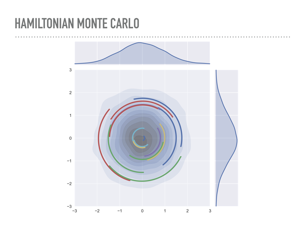
These ideas inspired an approach from physics, though, to use gradient information to travel through this typical set to distant regions. Michael Betancourt has a wonderful talk on the physics of this you can see online or when he comes to town. Intuitively, we are going to put our current position into orbit, using the probability distribution as a gravitational field. So, instead of just sampling points in n dimensions, we will sample both points and momentum, in 2n dimensions. So we run out of dimensions awful quickly if we want to visualize this. Here, I am sampling a 1-dimensional normal distribution, which is on the x-axis, and choosing the momentum distribution to also be normal, which you can see on the y-axis. At each step, I sample from the momentum, evolve the system according to Hamilton’s equations, which we will discuss, for a while, then project back to the x-axis to get my sample. We repeat this to sample from our distribution. Each of the colored lines in the plot is one of these Hamiltonian paths. |

|
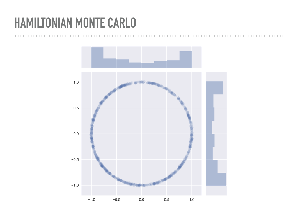
Here are 1,000 draws from the donut distribution we saw earlier, drawn with PyMC3 using a Hamiltonian sampler. Notice that we never resample the same point multiple times, so the samples are a little more diffuse. I’ll note that this took about twenty times as long as the Metropolis samples earlier. |
|
You can also see that HMC does fine with the skinnier donut. Intuitively, HMC is using gradient information to move through the pdf, which allows it to sample so efficiently. These samples were another ten times slower than the previous draws. |

|
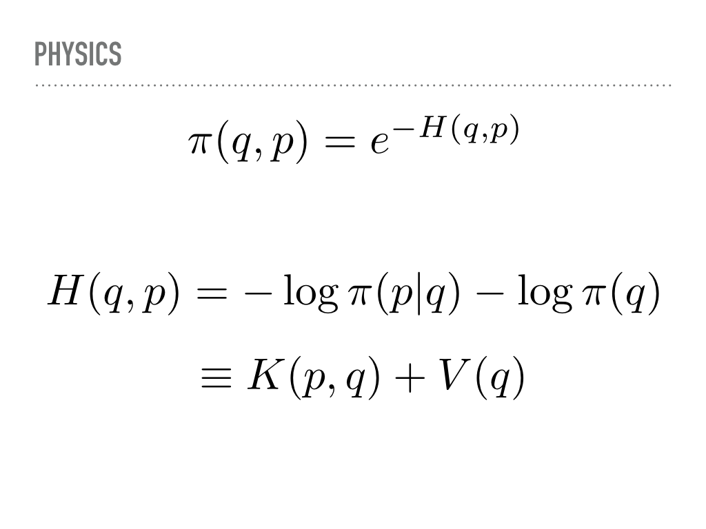
So what is going on mathematically? As I mentioned, we lift our position q to add some momentum p. This also lifts our pdf into a joint density function. We can factor this joint pdf so that when we marginalize the momentum, we are back to the desired distribution. This corresponds to the projection to the x-axis earlier. Notice also that we are stuck with π(q), but get to choose the conditional probability for the momentum. |
|
The Hamiltonian equations use an analogy to physics — if we have an electric or gravitational field and wish to move a particle through that field while conserving energy, how do the position and momentum change? We work in a log space, and so our probability distribution decomposes in this metaphor into a sum of kinetic energy, depending on position and momentum, and potential energy, which only depends on the position. |

|
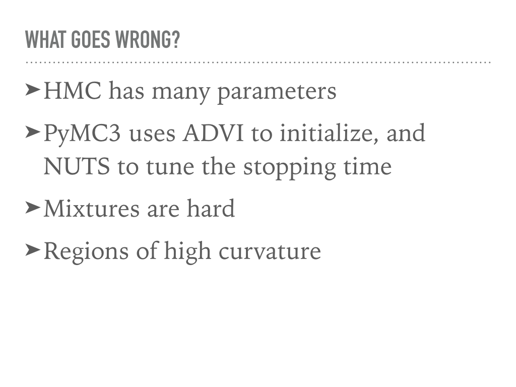
These are Hamilton’s equations. They let us know how to evolve the position and momentum. Once again, there is some mathematical bookkeeping I will not show, but every proposal made by integrating along these paths will be accepted, and we can integrate for arbitrarily long times to explore the different parts of the distribution. The current state of the art method in PyMC3 uses a “No-U-Turn” sampler that provides a rule for how long to follow a Hamiltonian path. Michael Betancourt has recently put that rule onto more solid theoretical footing, and there is a Google Summer of Code project working at using some of Betancourt’s ideas to achieve a more optimal stopping time in PyMC3. |
|
There are still plenty of problems, and we are still experimenting! A year ago, cutting edge for the library was its implementation of the No-U-Turn sampler, which was three years old at the time. Currently, there are at least three algorithms published in the past year which are under current development (OPVI, SGHMC, SMC). As mentioned, Metropolis-Hastings is still commonly used in practice, partly because it has so few knobs. PyMC3 will automatically use a reasonably tuned Hamiltonian sampler, but there are still plenty of places where this runs into trouble. The goal of a library like PyMC3 is to allow a researcher to design a model, then sample from it. The more parameters we can set automatically and optimally, the more useful the library will be. In cases where it cannot do this, we try to warn the user specifically of the problem and possible solutions. |
|
|
|
|
Learn More
PyMC3 |
AcknowledgementsThanks to Predrag Gruevski, Eugene Yurtsev, and Karin Knudson for feedback, discussion, and editing help, and to Jordi Diaz and Katherine Bailey for organizing and hosting the talk. |
|