Maximal Couplings

Definition

A maximal coupling between two distributions \(p\) and \(q\) on a space \(X\) is a distribution of a pair of random variables \((X, Y)\) that maximizes \(P(X = Y)\), subject to the marginal constraints \(X \sim p\) and \(Y \sim q\).

A few things about this definition we should pick out before going forwards:

1. This is a statement about making a joint distribution given two marginal distributions. For a great introduction to how to manipulate correlations while specifying marginal distributions, see Thomas Wiecki's nice post on copulas here.
2. The definition makes no claim that a maximal coupling is unique, and in fact, it is not.
3. This maximizes \(P(X=Y)\), so if we are thinking about applications, we had better make sure that \(X = Y\) even makes sense: \(p\) and \(q\) should be distributions over the same stuff.

Sampling from a maximal coupling

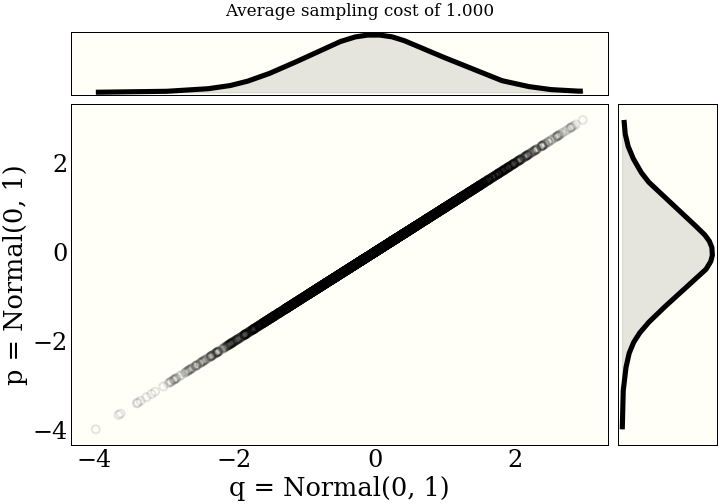
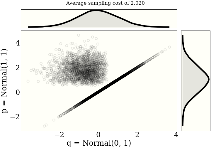
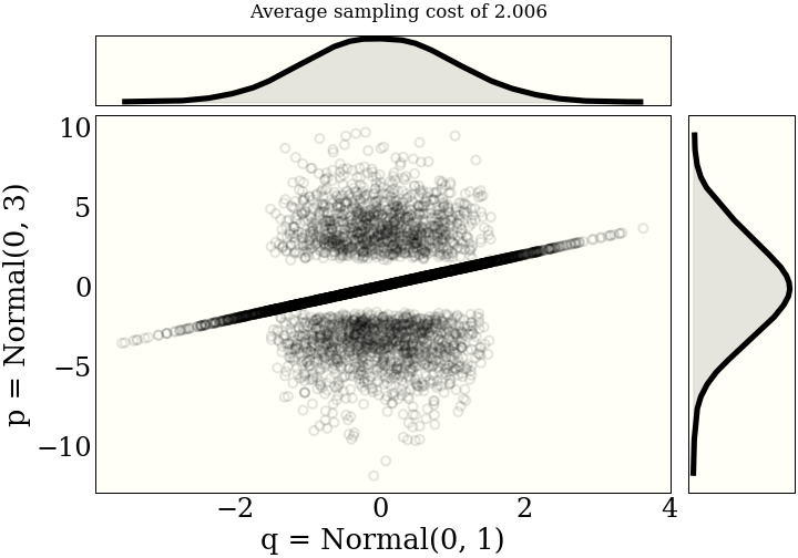
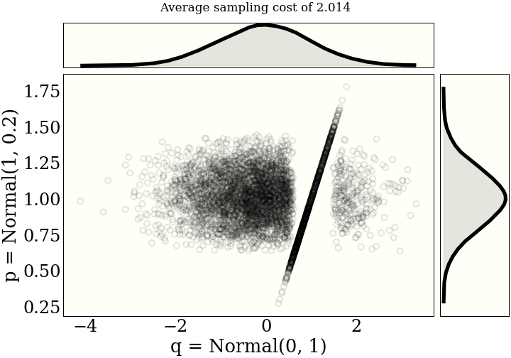
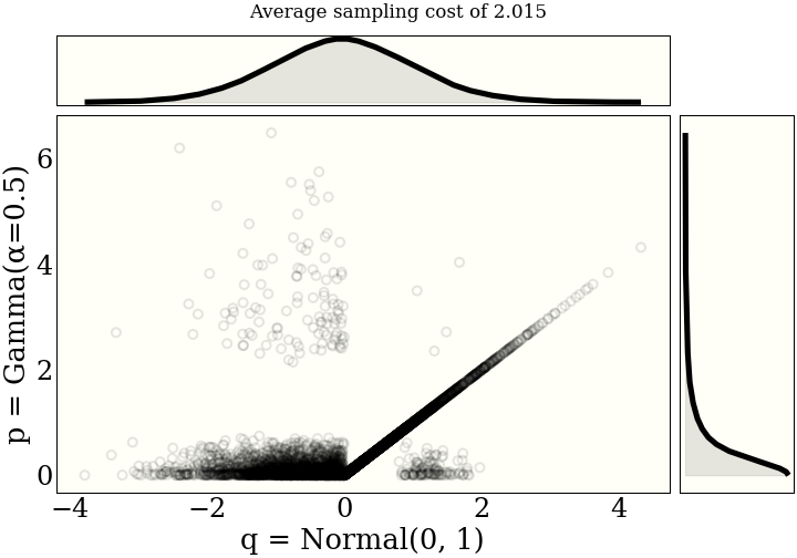
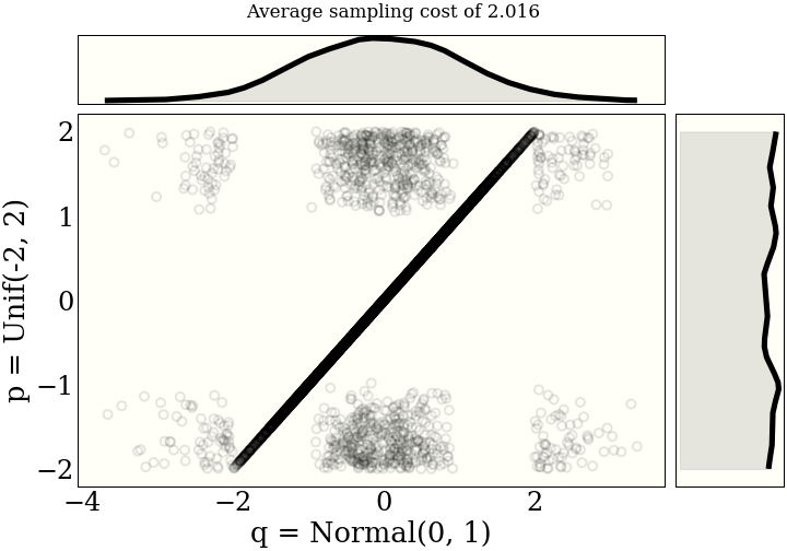
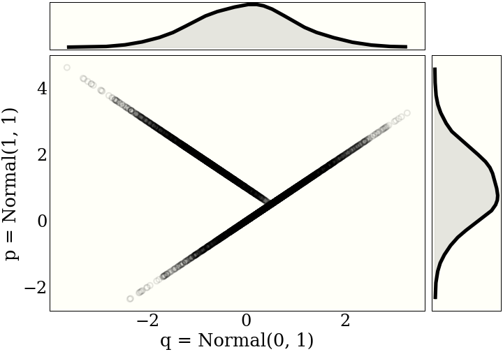
It helps the intuition to see a few examples of maximal couplings. Each figure includes the average "cost" of sampling from the joint distribution, as described in the paper.One unit of "cost" is a draw from either distribution, and a (log) probability evaluation from both distributions. So one draw, two evaluations.

Using this Python library, these distributions are generated using code like

import scipy.stats as st
from couplings import maximal_coupling

q = st.norm(0, 1)
p = st.norm(1, 1)

points, cost = maximal_coupling(p, q, size=5_000)

See below for details of what maximal_coupling is actually doing.

⊕This is a maximal coupling of two standard normal distributions. It makes sense that if the marginal distributions are the same and you want to maximize \(P(X=Y)\), then every draw from the joint distribution has the same value for \(X\) and \(Y\).

⊕This is a maximal coupling of two normal distributions with different means, but the same standard deviation, and it is starting to get interesting.

⊕This is a maximal coupling of two normal distributions with different standard deviations, but the same mean. Despite the somewhat bizarre looking joint distributions, note that this satisfies the definition of a maximal coupling.

⊕Here we have a different mean and a different variance.

⊕This is a maximal coupling of two distributions that have different support: the normal distribution could be any real number, but the gamma distribution is always positive.

⊕This is a maximal coupling of a uniform distribution and a normal distribution. I just thought this looked neat.

How does it work?

Here is a pseudocode implementation that happens to work in Python, and corresponds to algorithm 2 in Unbiased Markov Chain Monte Carlo with Couplings.

⊕In the actual library note that this is all vectorized, and the code is optimized a bit more. We also keep track of the cost of running the algorithm: the first return takes one sample and two pdf evaluations, which is one "cost" unit. The while loop also takes one "cost" each time through.

def maximal_coupling(p, q):
    X = p.sample()
    W = rand() * p(X)
    if W < q(X):
        return X, X
    else:
        while True:
            Y = q.sample()
            W = rand() * q(Y)
            if W > p(Y):
                return X, Y

Also, you can see why we might expect that \(X = Y\) at least some of the time due to the first if statement above, though that is certainly not a proof that this algorithm is correct. The interested/motivated reader can find a proof that this creates a maximal coupling by looking at the reference above.

Other maximal couplings

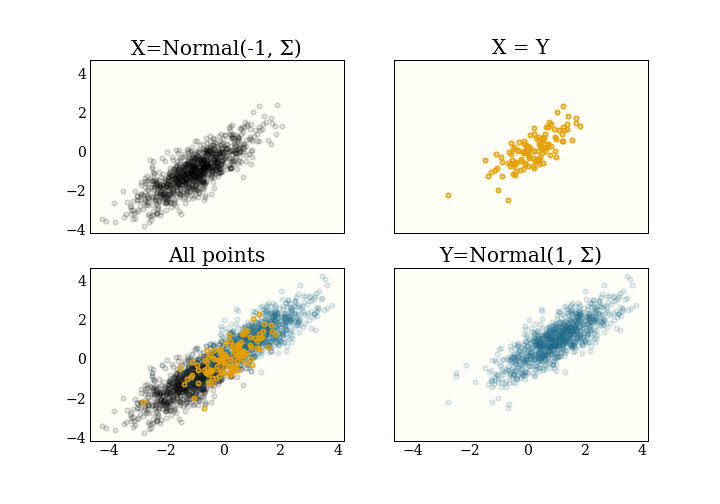
In the above algorithm, conditional on \(X \ne Y\), \(X\) and \(Y\) are independent. For reasons that are helpful later, we might instead use a maximal coupling that correlates \(X\) and \(Y\). It turns out to be particularly useful in the context of Metropolis-Hastings, to specialize this algorithm to the special case where \(p\) and \(q\) are given by $$ \begin{eqnarray} p &=& \mathcal{N}(\mu_1, \Sigma) \\ q &=& \mathcal{N}(\mu_2, \Sigma) \\ \end{eqnarray} $$ Specifically, in this case, \(\Sigma\) is the covariance matrix for the proposal distribution, and \(\mu_j\) is the current position of the two "coupled" chains. It is not important to understand that yet.

This is called a reflection maximal couplingThis is also implemented in the coupling library, in a very efficient (vectorized) manner. The implementation is pretty tricky, but well tested and fast, since it forms the backbone for much of the unbiased MCMC part of the library., and looks even more ridiculous. Note that the distributions need to be (multivariate) normals, and the covariances (standard deviations) have to be the same, so we are just changing the means.

⊕A reflection maximal coupling of two normals with slightly different means. Notice that when \(X \ne Y\), the draws are not independent.

⊕We saw this image earlier, but I want to show it again to emphasize that maximal couplings are not unique.

⊕This is an example of some two dimensional reflection maximal couplings. Note that we can only see the marginal distributions here, since we are dealing with four dimensions. I am not sure how illuminating this is, but it is traditional to take a stab at visualizing four dimensions if you have a chance to do so. The covariance matrix here creates a fairly correlated Gaussian.

Conclusion

In itself, we might just view this as a statistical curiosity, and use it to think about how flexible a joint distribution can be, even after fixing the marginal distributions. In followup posts, I will write more about how maximal couplings are used for unbiased MCMC.